One must first choose a suitable scaling scheme to use for a spectrum that consists neither of incoherent noise nor of completely coherent sine waves, but of modes of finite lifetime, superimposed on a non-negligible noise background. The situation is further complicated because, in practice, a substantial fraction of the data in the time series is missing: our best 2-month spectrum so far has 94 per cent fill, but in some early years the best 2-month fills were around 25 per cent (early to mid 1980 s). For frequency measurements, of course, the scaling can be arbitrary, but in order to compare mode amplitudes obtained from different spectra the scaling needs to be carefully considered. There are two main methods of scaling power spectra: "power per unit frequency'' and "equivalent sine wave''. In the former method, the total power in the spectrum is equal to the sum of the squares of the velocity residuals - or, in our case, to the sum of squares of the residuals divided by the fill to allow for the missing data. This method is appropriate when comparing incoherent noise levels.
When there are zero-valued residuals in the time series - owing to the presence of gaps - power will be re-distributed into sidebands characteristic of the Fourier transform of the resulting window function. The power in the central peak will therefore be reduced. The equivalent sine-wave scaling scheme compensates for this, by dividing again by the fill, to give an estimate of the power in the oscillatory signal that is independent of the window function. This method is appropriate for estimating the power in a given signal.
The window function can usefully be characterized by generating an
artificial spectrum in which the real data in a time series are
replaced by a single sinusoid of a frequency such that it appears in
a single bin of the power spectrum. There is generally a dominant
24-hour period due to the regular interruption of the data by night,
which gives rise to a series of sidelobes associated with each peak,
spaced at 1/day or approximately 11.57 ![]() Hz. In the analysis of
the low-
Hz. In the analysis of
the low-![]() p-mode spectrum, where the modes occur in pairs
separated by about 5 to 15
p-mode spectrum, where the modes occur in pairs
separated by about 5 to 15 ![]() Hz, this can be a serious problem, as
one peak may overlap with the sidelobe of its neighbour. With a
multi-station network, although some remnant of the twenty-four hour
period persists, the breaks are more random and the 1/day sidelobes
are greatly reduced in size. Figure 3 (click here) shows typical window
function transforms for a one-station and a six-station time series.
In our best six-station spectra, the sidelobes have all but
disappeared into the window-function noise.
Hz, this can be a serious problem, as
one peak may overlap with the sidelobe of its neighbour. With a
multi-station network, although some remnant of the twenty-four hour
period persists, the breaks are more random and the 1/day sidelobes
are greatly reduced in size. Figure 3 (click here) shows typical window
function transforms for a one-station and a six-station time series.
In our best six-station spectra, the sidelobes have all but
disappeared into the window-function noise.
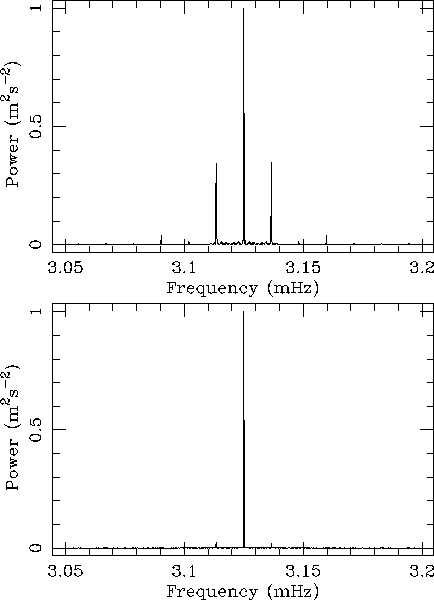
Figure 3: Window function power spectrum for
May through June 1996. Here, a sine wave with period 320 s and
amplitude ![]() has been forced through each window
function. Top: Tenerife only, fill 32 per cent. Bottom: Six stations,
fill 78 per cent. The ordinate is equivalent sine-wave scaled
has been forced through each window
function. Top: Tenerife only, fill 32 per cent. Bottom: Six stations,
fill 78 per cent. The ordinate is equivalent sine-wave scaled
In addition to the discrete sidelobes, the window function contains background noise and some power in the wings of the central peak. The broadening of the central peak, which is particularly severe if there are long gaps in the data, can corrupt the measurement of mode strengths and must be corrected for when comparing mode amplitudes between spectra. This correction has been discussed in detail by Elsworth et al. (1993). The correction applied for 1/day sidelobes is discussed below under the heading of "sidelobe fitting''.
The ragged appearance of the power spectrum of the modes arises from the stochastically excited nature of the oscillations and the fact that each Fourier spectrum is only an estimate, or realization, of the true spectrum, where the power in each bin consists of the underlying spectrum multiplied by a random number distributed as chi-squared with two degrees of freedom (Duvall & Harvey 1986; Anderson, Duvall & Jefferies 1990). If a large number of such realizations were averaged together, a better estimate of the true spectrum would be obtained, with errors tending to a Gaussian distribution. However, unlike observers studying the high-degree modes by resolving the image of the Sun, we have only a few dozen modes and two to three dozen spectra of reasonable quality to work with. In very early work the repeating pattern of the spectrum made it useful to average together corresponding portions of the spectrum at different frequencies. However, more detailed examination of well-resolved spectra reveal that the properties (including the repeat interval) of the spectrum vary considerably with frequency: the averaging of different frequencies is therefore of limited use for accurate work. Moreover, the properties of the spectrum vary with solar activity (e.g., Libbrecht & Woodard 1990, 1991; Rhodes et al. 1993; Elsworth et al. 1993, 1994b; Regulo et al. 1994): averages of many spectra from different epochs obscure this information and must be treated with caution. We therefore work mainly with individual spectra, or occasionally with the mean of two spectra close together in time.
As discussed by Anderson, Duvall & Jefferies, one approach to the
treatment of individual spectra is to fit the model parameters to the
peaks using a "maximum likelihood'' method with the appropriate
statistics, rather than normal least-squares fitting, which assumes a
Gaussian distribution of the data points about the model. We have
recently started to use this method in studies of high-resolution
spectra. In our earlier work (Elsworth et al. 1990a,b, 1991,
1993, 1994), however, we have adopted a different approach. The power
spectra are first smoothed using a weighted moving mean
(Pollard
1977). Pairs of peaks are then fitted to a model function using
non-linear least-squares methods. A frequency range of about 50
![]() Hz (about 250 frequency bins) is used to fit an
Hz (about 250 frequency bins) is used to fit an ![]() ,
,
![]() pair, and a range of 70
pair, and a range of 70 ![]() Hz for an
Hz for an ![]() ,
, ![]() pair. As was discussed in our publication on mode strengths
(Elsworth et al. 1993), the smoothing does introduce systematic
errors in the height and width of the fitted peaks, but these can be
corrected for. We have attempted to deconvolve the smoothing function
by using the same smoothing on the model function as was used on the
data, but this was found not to be effective. We have found
empirically that the smoothing function chosen has no effect on a
Lorentzian peak profile until the frequency range over which the
smoothing is carried out exceeds the full width at half maximum of
the peak. Thereafter the width of the peak is increased by the
addition in quadrature of the effective width of the smoothing
function, which is slightly less than one third of the full range of
the function, while its height decreases.
pair. As was discussed in our publication on mode strengths
(Elsworth et al. 1993), the smoothing does introduce systematic
errors in the height and width of the fitted peaks, but these can be
corrected for. We have attempted to deconvolve the smoothing function
by using the same smoothing on the model function as was used on the
data, but this was found not to be effective. We have found
empirically that the smoothing function chosen has no effect on a
Lorentzian peak profile until the frequency range over which the
smoothing is carried out exceeds the full width at half maximum of
the peak. Thereafter the width of the peak is increased by the
addition in quadrature of the effective width of the smoothing
function, which is slightly less than one third of the full range of
the function, while its height decreases.
We have carried out numerous tests in which artificial spectra,
generated from known parameters, were smoothed and fitted in the same
way as the real data. Although individual realizations behave in very
different ways, the effect of the smoothing on the average parameters
can be predicted from the behaviour of a simple Lorentzian peak under
the same amount of smoothing, provided that the smoothing is not
performed over too wide a range compared with the peak width. In
practice, for two-month spectra, we use between 7 and 49 bins (about
1.5 to 10 ![]() Hz), using the heavier smoothing for the wider modes
at the high-frequency end of the spectrum. The fitted peak parameters
are corrected for the effect of smoothing as follows. The width
obtained from the fit is first corrected for the effect of smoothing
by subtracting in quadrature the effective width of the smoothing
function. A Lorentzian peak of this corrected width and known height
is then smoothed and fitted in the same way as the real data, in
order to estimate the correction to be applied to the peak height. By
comparing the results from the same spectrum fitted with different
amounts of smoothing, we have verified that this procedure
satisfactorily removes the systematic effects of smoothing.
Hz), using the heavier smoothing for the wider modes
at the high-frequency end of the spectrum. The fitted peak parameters
are corrected for the effect of smoothing as follows. The width
obtained from the fit is first corrected for the effect of smoothing
by subtracting in quadrature the effective width of the smoothing
function. A Lorentzian peak of this corrected width and known height
is then smoothed and fitted in the same way as the real data, in
order to estimate the correction to be applied to the peak height. By
comparing the results from the same spectrum fitted with different
amounts of smoothing, we have verified that this procedure
satisfactorily removes the systematic effects of smoothing.
The model function used to fit a pair of neighbouring peaks consists
of two Lorentzian profiles, for which the adjustable parameters are
the height h, the full width at half-maximum ![]() , and the
central frequency
, and the
central frequency ![]() , on a flat background of which the size b
is also an adjustable parameter. The power,
, on a flat background of which the size b
is also an adjustable parameter. The power, ![]() , in each single
Lorentzian component, is given by
, in each single
Lorentzian component, is given by
![]()
Associated with each peak is a pair of symmetrical sidelobes at
11.57 ![]() Hz on either side of the central peak. The sidelobes are
assumed to have the same width and Lorentzian shape as the central
peak, but their height relative to the main peak is left as an
adjustable parameter for each peak. The relative height of the
sidelobes can vary significantly from one peak to another. This is
partly because of interference with neighbouring modes and noise, but
we believe that a real effect is also involved: the amplitude of
individual modes can vary dramatically from one week to the next, so
that if a particular mode happens to have been strong for a period
when only one or two stations were producing good data, it will
appear to have stronger sidelobes than one that was strong when the
network was running well. A more rigorous method of allowing for the
sidelobes would be to convolve the model function with the known
window function spectrum at each step of the minimization. This form
of deconvolution would be much more expensive in computing time, and
makes no allowance for the sidelobe variability discussed above.
Hz on either side of the central peak. The sidelobes are
assumed to have the same width and Lorentzian shape as the central
peak, but their height relative to the main peak is left as an
adjustable parameter for each peak. The relative height of the
sidelobes can vary significantly from one peak to another. This is
partly because of interference with neighbouring modes and noise, but
we believe that a real effect is also involved: the amplitude of
individual modes can vary dramatically from one week to the next, so
that if a particular mode happens to have been strong for a period
when only one or two stations were producing good data, it will
appear to have stronger sidelobes than one that was strong when the
network was running well. A more rigorous method of allowing for the
sidelobes would be to convolve the model function with the known
window function spectrum at each step of the minimization. This form
of deconvolution would be much more expensive in computing time, and
makes no allowance for the sidelobe variability discussed above.
A commonly used method for extracting mode parameters from power
spectra is to use a maximum-likelihood estimator that takes into
account the exponential distribution of the data about the underlying
spectrum. As discussed above, we have found our own smoothing and
least-squares fitting methods adequate for obtaining frequency
measurements from 2-month power spectra. However, in most of this
analysis we have neglected the rotational splitting of the modes of
![]() and treated all modes as single Lorentzian peaks. As the
rotational splitting is not clearly resolved - particularly in
2-month spectra - for frequencies above about 2.2 mHz, and there is
neither strong empirical evidence for, nor any theoretical reason to
expect (at least from a simple model) asymmetries in the amplitudes
of splitting components, this seemed to us a reasonable
approximation. However, when we wish to analyse higher-resolution
spectra to derive the rotational splitting of lower-frequency modes,
the smoothing method becomes less appropriate. As discussed in
Elsworth et al. (1995a), we have therefore chosen to use
maximum-likelihood estimation on power spectra covering periods up
to, for example, 16 months, with model functions that explicitly
include the splitting components at the theoretically expected
amplitude ratios calculated by Christensen-Dalsgaard (1989).
To satisfy the statistical requirements of some aspects of the fitting
procedure, we vary the logarithms of some of the parameters,
rather than the parameters themselves.
and treated all modes as single Lorentzian peaks. As the
rotational splitting is not clearly resolved - particularly in
2-month spectra - for frequencies above about 2.2 mHz, and there is
neither strong empirical evidence for, nor any theoretical reason to
expect (at least from a simple model) asymmetries in the amplitudes
of splitting components, this seemed to us a reasonable
approximation. However, when we wish to analyse higher-resolution
spectra to derive the rotational splitting of lower-frequency modes,
the smoothing method becomes less appropriate. As discussed in
Elsworth et al. (1995a), we have therefore chosen to use
maximum-likelihood estimation on power spectra covering periods up
to, for example, 16 months, with model functions that explicitly
include the splitting components at the theoretically expected
amplitude ratios calculated by Christensen-Dalsgaard (1989).
To satisfy the statistical requirements of some aspects of the fitting
procedure, we vary the logarithms of some of the parameters,
rather than the parameters themselves.
The calculation of formal errors for this kind of fit, where neither the parameters nor (because of incomplete fill) the data points are completely independent, is complicated. We have in the past chosen to use the scatter of many determinations from independent spectra to estimate the errors of the peak parameters. This becomes more difficult with long spectra, of which we have only a few examples.
A thorough discussion of the errors in BiSON data can be found in Chaplin et al. (1996e), in which we outline our reservations regarding the use of formal uncertainties.