Results of the observations are presented in Figs. 1 (click here)-3 (click here) as residual light curves (numerical values are available upon request in the form of an ASCII file). Residuals are defined as:
![]()
where <S> is the mean flux density. Figure 1 (click here) shows
light curves with temporal resolution of ![]() minutes.
Figures 2 (click here) and 3 (click here) contain residuals with resolution of 1 day
and 1 month, respectively. Residual curves corresponding to steep-spectrum
sources have been included in the figures for comparison.
minutes.
Figures 2 (click here) and 3 (click here) contain residuals with resolution of 1 day
and 1 month, respectively. Residual curves corresponding to steep-spectrum
sources have been included in the figures for comparison.
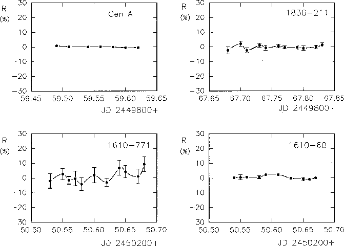
Figure 1: Residual light curves for intraday observations
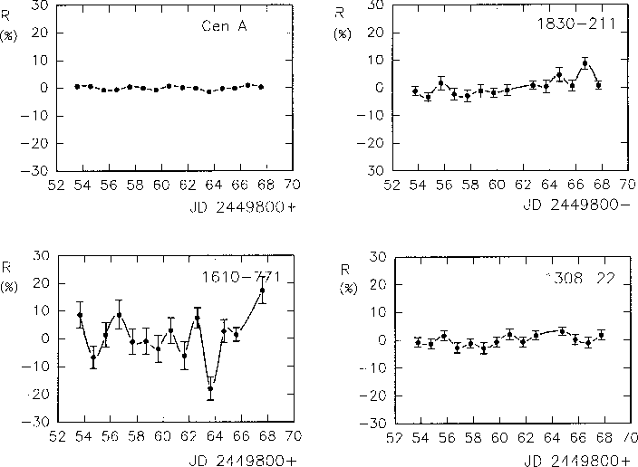
Figure 2: Residual light curves for interday observations

Figure 3: Residual light curves for intermonth observations
In order to check the presence of variability in the different light
curves a ![]() -test with a confidence level of 99.9% was applied. No
variability within the measurement errors was detected at intraday resolution.
Interday variability was present in PKS 1610-771.
Cen A seems to be non-variable over timescales of weeks or
less at 1.4 GHz. However, variations of
-test with a confidence level of 99.9% was applied. No
variability within the measurement errors was detected at intraday resolution.
Interday variability was present in PKS 1610-771.
Cen A seems to be non-variable over timescales of weeks or
less at 1.4 GHz. However, variations of ![]() were detected over
timescales of months. Two bursts can be observed in the light curve shown
in Fig. 3 (click here). PKS 1610-771 was also variable over large timescales.
were detected over
timescales of months. Two bursts can be observed in the light curve shown
in Fig. 3 (click here). PKS 1610-771 was also variable over large timescales.
The observed variability can be characterized by a percentage fluctuation index:
![]()
Fluctuations of the steep-spectrum sources included in the sample for
control purposes were then interpreted as spurious variability introduced by the
observing system. If ![]() is the largest fluctuation index of calibration
sources during a campaign with temporal resolution
is the largest fluctuation index of calibration
sources during a campaign with temporal resolution ![]() , then the
real variability of the source under study can be measured by an amplitude
, then the
real variability of the source under study can be measured by an amplitude
![]() given by (e.g. Quirrenbach et al. 1992):
given by (e.g. Quirrenbach et al. 1992):
![]()
Variability parameters for the three sources of our sample are given in
Table 3 (click here): source name, number of points in the light curve, mean
flux density, result of the ![]() -test (V: variable, NV: non variable),
fluctuation index, variability amplitudes, associated timescales, activity
parameter
-test (V: variable, NV: non variable),
fluctuation index, variability amplitudes, associated timescales, activity
parameter ![]() , and the slope of the corresponding structure function
(see below), from left to right. Typical values of
, and the slope of the corresponding structure function
(see below), from left to right. Typical values of ![]() are
are ![]() ,
except for the intraday observations of PKS 1610-771 where larger values
were observed (
,
except for the intraday observations of PKS 1610-771 where larger values
were observed (![]() ).
).

Table 3: Variability parameters
The timescales in Table 3 (click here) were determined by means of the first-order structure functions introduced by Simonetti et al. (1985):
![]()
where R(t) is the residual at time t and the average is
taken over all pairs of observations with time lag T. The maxima in the
![]() plane characterize the timescales of a given
source. The slope
plane characterize the timescales of a given
source. The slope ![]() of the structure functions can be used to
investigate the nature of the underlying physical process (e.g.
Qian et al. 1995). Structure functions for the light curves
with variability are shown in Fig. 4 (click here).
The structure function of PKS 1830-211 at interday resolution is also
shown in this figure.
of the structure functions can be used to
investigate the nature of the underlying physical process (e.g.
Qian et al. 1995). Structure functions for the light curves
with variability are shown in Fig. 4 (click here).
The structure function of PKS 1830-211 at interday resolution is also
shown in this figure.
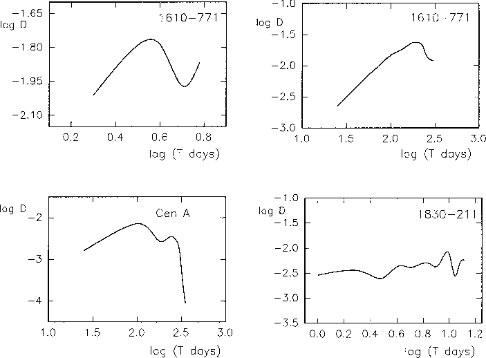
Figure 4: First-order structure functions
PKS 1830-211 has been classified as NV due to its flat structure
function and the result of the ![]() -test. However, a small
variability amplitude can be assigned to the interday and
intermonth light curves owing to a one-point deviation in each
curve (see Figs. 2 (click here), 3 (click here) and 4 (click here)). These amplitudes
have been included in Table 2 (click here). The possibility of a real variation
with a timescale of
-test. However, a small
variability amplitude can be assigned to the interday and
intermonth light curves owing to a one-point deviation in each
curve (see Figs. 2 (click here), 3 (click here) and 4 (click here)). These amplitudes
have been included in Table 2 (click here). The possibility of a real variation
with a timescale of ![]() cannot be ruled out.
cannot be ruled out.