In this section we determine the error budget of the processing and
estimate the quality of the determination of ![]() and B or
and B or ![]() according to the geometry of the double star.
according to the geometry of the double star.
In the simulation we have generated few relatively short period binaries of various separations and computed several series of observations, using the time sequences found in the Hipparcos data sets.
According to the theoretical approach of the preceding sections, we assume that the
quality of the determination of
![]() and B or of their difference depends primarily on the three following
parameters:
and B or of their difference depends primarily on the three following
parameters:
For the sake of simplicity,
each simulation refers to a particular semi-major axis a, which is
by far the most important single geometric orbital parameter in this study. As for
the other elements, each final output of the simulation is an average value (or more
precisely a median) of 30 realistic cases, each resulting from a random drawing of the
five remaining orbital elements, namely the inclination
i, the eccentricity
e, the position angles ![]() and
and ![]() of the ascending node and of the
periastron, and the epoch T. The details of this selection are really unimportant
here and are not given.
of the ascending node and of the
periastron, and the epoch T. The details of this selection are really unimportant
here and are not given.
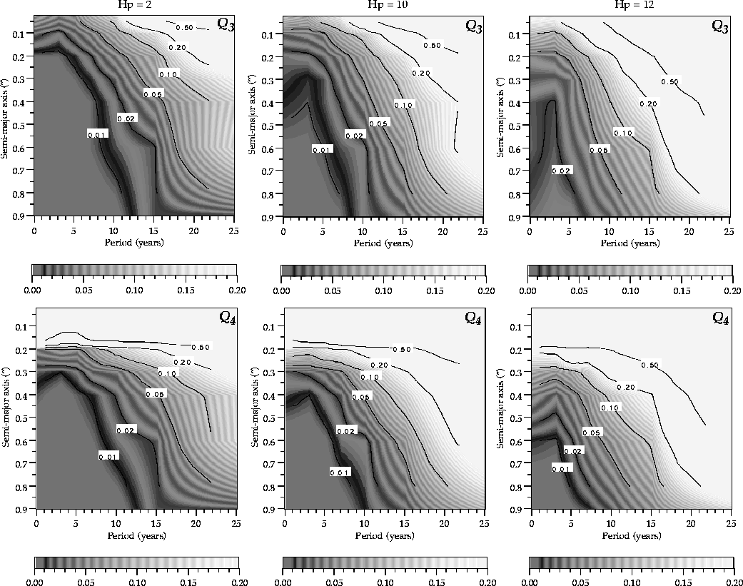
Figure 7: Some results of the simulation ![]() (stars with
(stars with ![]() ) for a global magnitude of
2 (left), 10 (middle) and 12 (right). The indice
) for a global magnitude of
2 (left), 10 (middle) and 12 (right). The indice ![]() (on the top) represents the
standard deviation of
(on the top) represents the
standard deviation of ![]() issued from the processing, while
issued from the processing, while
![]() (on the bottom) represents the standard deviation on the mass fraction B
alone. Even
for the shorter periods and the lowest magnitudes, it remains impossible to determine
(on the bottom) represents the standard deviation on the mass fraction B
alone. Even
for the shorter periods and the lowest magnitudes, it remains impossible to determine ![]() and B separately if the semi-major axis is less than 02. The constraint on the period
is also crucially strengthened as the brightness decreases
and B separately if the semi-major axis is less than 02. The constraint on the period
is also crucially strengthened as the brightness decreases
The primary goal of the simulation is to determine in the space semi-major
axis-period, the regions where a separate determination of the mass- and
intensity-ratio is achievable and where only the scale of the photocentric orbit will
be obtained. As a second objective, the simulation should also allow to analyze
the effects of the choice of the initial values
![]() and
and ![]() on the convergence of the procedure, particularly in the cases of
strong non-linearity (appearing when
on the convergence of the procedure, particularly in the cases of
strong non-linearity (appearing when ![]() is small and the separation is about
half a grid step). The third one, which is commonplace, is to help in the writing and
testing of the software.
is small and the separation is about
half a grid step). The third one, which is commonplace, is to help in the writing and
testing of the software.
The values of the input parameters for each run,
a, P and ![]() , are given in Table 1 (click here). This choice leads to simulate 147
basic cases (
, are given in Table 1 (click here). This choice leads to simulate 147
basic cases (![]() values), each giving rise to at least 30 random
simulations as said before.
values), each giving rise to at least 30 random
simulations as said before.
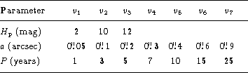
Table 1: Simulation's grid: values ![]() of the three input parameters
of the three input parameters
As for the other parameters they are selected as follows: the actual value of the mass
fraction
B has no effect on the results, and thus was fixed to 0.3 in all cases, or
equivalently ![]() . Regarding
. Regarding ![]() , apart from the
very specific case with
, apart from the
very specific case with ![]() considered in Sect. 5.3, most of the
tests were run with
considered in Sect. 5.3, most of the
tests were run with ![]() or
or ![]() . Changing
. Changing ![]() between 0.3 and 3 showed conclusively that the results were not very sensitive to
any particular choice in this range.
The number of observations, the position of the simulated stars on the sky and the
distribution of the scanning angles in orientation and time are chosen in order to
respect the characteristics of the Hipparcos scanning law. The distance GH from
the centre of mass to the
hippacentre was perturbed for each observation by a gaussian noise with a standard
deviation function of the magnitude of the simulated system. The updating of
between 0.3 and 3 showed conclusively that the results were not very sensitive to
any particular choice in this range.
The number of observations, the position of the simulated stars on the sky and the
distribution of the scanning angles in orientation and time are chosen in order to
respect the characteristics of the Hipparcos scanning law. The distance GH from
the centre of mass to the
hippacentre was perturbed for each observation by a gaussian noise with a standard
deviation function of the magnitude of the simulated system. The updating of
![]() and B during the iterations depended on their observed correlation. For
sufficiently large
a,
and B during the iterations depended on their observed correlation. For
sufficiently large
a, ![]() and B are nearly independent and were separately updated.
Otherwise, the relevant information is contained in the difference
and B are nearly independent and were separately updated.
Otherwise, the relevant information is contained in the difference
![]() and the processing ended up only with a correction
and the processing ended up only with a correction ![]() .
Hence, the updating was realized by splitting it into two
unequal parts, as:
.
Hence, the updating was realized by splitting it into two
unequal parts, as:
![]()
where the coefficient ![]() was
generally taken equal to 0.8, to allow for the fact that for real systems
was
generally taken equal to 0.8, to allow for the fact that for real systems
![]() is as a rule better known than B. We observed that no more than two or
three iterations were needed to reach the convergence.
To start the solution algorithm we have taken
is as a rule better known than B. We observed that no more than two or
three iterations were needed to reach the convergence.
To start the solution algorithm we have taken ![]() and
and ![]() , which gives a difference of 0.1 on
, which gives a difference of 0.1 on ![]() between the true value and the
initial value fed into the software.
between the true value and the
initial value fed into the software.
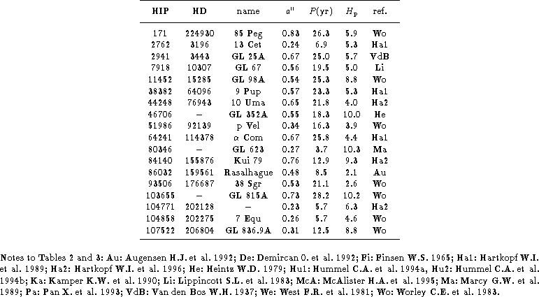
Table 2: List of candidate stars with possible determination of both the mass
and intensity ratio
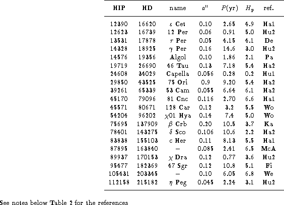
Table 3: List of candidate stars with likely determination of the
scale of the
photocentric orbit
There are basically two indicators available to assess the solutions:
We derived for each of the 147 basic
cases, five different indicators, denoted
![]() to
to ![]() .
The first two are external indicators of quality, based on the comparison
between the input and output values of the intensity and mass ratio, respectively
.
The first two are external indicators of quality, based on the comparison
between the input and output values of the intensity and mass ratio, respectively
![]() and
and ![]() :
:
![]()
![]()
where the notation Med(X) stands for the median of the set X, with ![]() , for
the 30 simulated cases (Sect. 5.1). The
numerical factor in 11-12 follows from the mathematical expectation of the
median of the absolute value of a gaussian random variable of zero mean and standard
deviation
, for
the 30 simulated cases (Sect. 5.1). The
numerical factor in 11-12 follows from the mathematical expectation of the
median of the absolute value of a gaussian random variable of zero mean and standard
deviation
![]() , which is such that Med
, which is such that Med![]() .
The remaining three indices are derived from the
variance-covariance matrix of the seven unknowns:
.
The remaining three indices are derived from the
variance-covariance matrix of the seven unknowns:
![]()
![]()
![]()
where ![]() is the standard deviation of x, and
is the standard deviation of x, and ![]() is the correlation coefficient between x and y. While
is the correlation coefficient between x and y. While ![]() and
and ![]() are directly derived from the fitting,
are directly derived from the fitting, ![]() is evaluated from the error
propagation as,
is evaluated from the error
propagation as,
![]()
The main results appear in Fig. 7 (click here) as maps with contour lines
for the indices ![]() and
and ![]() (the indices
(the indices ![]() and
and ![]() have also been plotted; As the corresponding
maps are very similar to
those of Fig. 7 (click here), they are not presented in this paper). The horizontal axes on each map represent the period
in years and the semi-major axis in arcsec, while the value of each of the indicators is
shown by the label of the contour lines.
To fully appreciate the significance of the results shown in Fig. 7 (click here), one must
first consider that the light area in the upper right of each diagram represents the
domain of orbital periods and orbit size, where no valuable information on
have also been plotted; As the corresponding
maps are very similar to
those of Fig. 7 (click here), they are not presented in this paper). The horizontal axes on each map represent the period
in years and the semi-major axis in arcsec, while the value of each of the indicators is
shown by the label of the contour lines.
To fully appreciate the significance of the results shown in Fig. 7 (click here), one must
first consider that the light area in the upper right of each diagram represents the
domain of orbital periods and orbit size, where no valuable information on ![]() and/or B can be extracted from the Hipparcos observations. Not surprisingly the size
of this domain increases with the star magnitude. On the contrary the dark patches
indicate the range of separations and orbital periods allowing the determination
of the mass and intensity ratio with an acceptable accuracy.
There is no hope to measure the mass
ratio with the Hipparcos data for separations less than 015, unless the
magnitude difference is well known. In the latter case the scale of the photocentric
orbit may yield a significant result even for a separation
and/or B can be extracted from the Hipparcos observations. Not surprisingly the size
of this domain increases with the star magnitude. On the contrary the dark patches
indicate the range of separations and orbital periods allowing the determination
of the mass and intensity ratio with an acceptable accuracy.
There is no hope to measure the mass
ratio with the Hipparcos data for separations less than 015, unless the
magnitude difference is well known. In the latter case the scale of the photocentric
orbit may yield a significant result even for a separation ![]() .
.
Let's come now to the limiting cases already mentioned in Sect. 2.3 when either ![]() or when the secondary is very faint.
The tests made on systems with large
or when the secondary is very faint.
The tests made on systems with large ![]() confirm the conclusion of Sect. 2.3;
No particular problem appears in this situation, corresponding to a classical
astrometric binary with an unseen companion. The mass ratio B is retrieved from the
absolute motion of the primary, and this, even for separations slightly smaller than in
the more common situation considered in the previous sections.
On the other hand, when the two components are of similar brightness, the solving
of the non linear system proved more difficult and required care in the choice of the
variables. Good solutions were
obtained only with periods shorter than 15 years when
confirm the conclusion of Sect. 2.3;
No particular problem appears in this situation, corresponding to a classical
astrometric binary with an unseen companion. The mass ratio B is retrieved from the
absolute motion of the primary, and this, even for separations slightly smaller than in
the more common situation considered in the previous sections.
On the other hand, when the two components are of similar brightness, the solving
of the non linear system proved more difficult and required care in the choice of the
variables. Good solutions were
obtained only with periods shorter than 15 years when ![]() and shorter
than 7 years for smaller values of a.
and shorter
than 7 years for smaller values of a.
According to the results of the simulation, it is possible to set up a list of
Hipparcos stars which are likely to be good candidates to such an analysis,
assuming the relative orbits are sufficiently well known. We have split this set
into two categories according to whether
![]() and
B may be separately determined or not. This two sets are given respectively in
Tables 2 (click here) and 3 (click here), where the values of the semi-major axis and the period are rounded.
When we start the processing on real data some stars will disappear and
from additional searchs in the literature we might spot new candidates.
The importance of the systems belonging to the second category should not be
underevalued; As the corresponding separations are quite small, one may find a
lot of objects with extremely short periods (less than 5 years), a very favourable
circumstance. One may also hope to know the magnitude difference from
ground-based observations, so that the mass fraction B will be also derived with a
good accuracy.
and
B may be separately determined or not. This two sets are given respectively in
Tables 2 (click here) and 3 (click here), where the values of the semi-major axis and the period are rounded.
When we start the processing on real data some stars will disappear and
from additional searchs in the literature we might spot new candidates.
The importance of the systems belonging to the second category should not be
underevalued; As the corresponding separations are quite small, one may find a
lot of objects with extremely short periods (less than 5 years), a very favourable
circumstance. One may also hope to know the magnitude difference from
ground-based observations, so that the mass fraction B will be also derived with a
good accuracy.