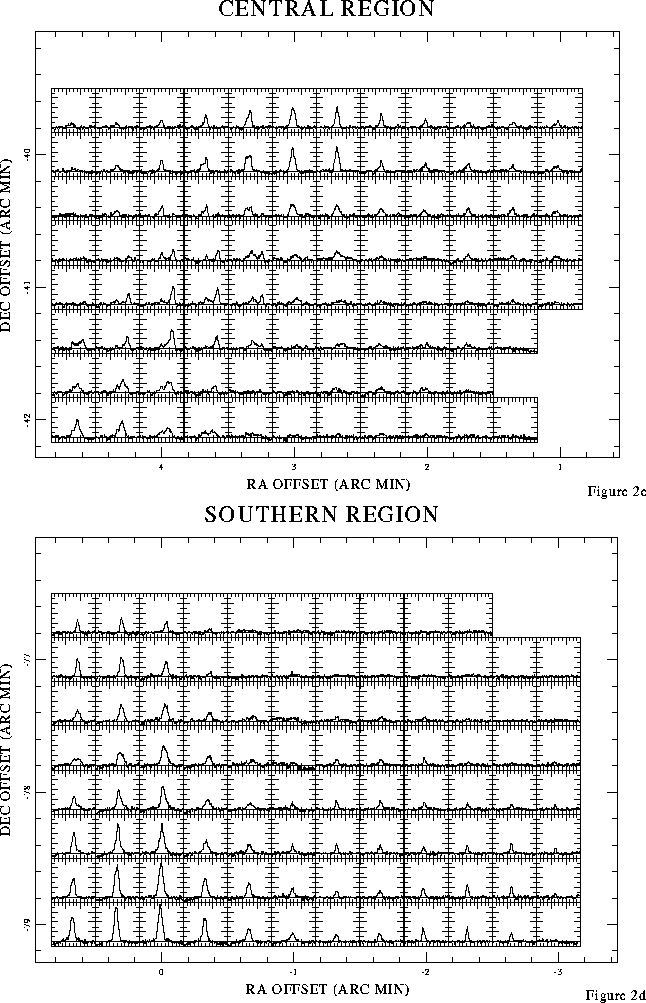
In Fig. 2 (click here), we show several sample spectra from both the Central
and Southern regions. The RA and DEC offsets are with respect to
![]() ,
, ![]() . These
spectra provide an idea of the quality of the data. In addition, we can
see how the line falls off from the cloud center to edge. Also,
we get an idea of how the line profiles change as one moves across
the cloud. The general appearance of the line profiles is similar
to that seen in Milky Way molecular clouds, especially those seen
in the outer Galaxy, where there is little confusion along the
line of sight (Mead & Kutner 1988). The major difference is
that the LMC lines are much weaker than the Galactic counterparts.
. These
spectra provide an idea of the quality of the data. In addition, we can
see how the line falls off from the cloud center to edge. Also,
we get an idea of how the line profiles change as one moves across
the cloud. The general appearance of the line profiles is similar
to that seen in Milky Way molecular clouds, especially those seen
in the outer Galaxy, where there is little confusion along the
line of sight (Mead & Kutner 1988). The major difference is
that the LMC lines are much weaker than the Galactic counterparts.
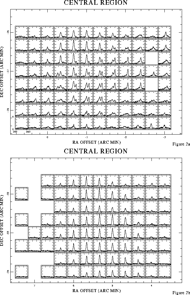
Figure 2: A selection of spectra from four (three in the Central
part and one in the Southern part) different parts of the region.
In each region we show a rectangular arrangement of spectra.
Boxes are on a half beamwidth grid. For each box the velocity and
temperature axes are the same, and are indicated in the sample
box in Fig. 2a.
(![]() ) offsets are from the reference position,
) offsets are from the reference position, ![]() ,
, ![]()
Contour maps of the overall CO emission are shown in Fig. 3 (click here). In
Fig. 3 (click here)a (Central region) and 3c (Southern region) we present
contour maps of peak ![]() at each position, and then, in Figs. 3b and
3d, contour maps of the integrated CO intensity,
at each position, and then, in Figs. 3b and
3d, contour maps of the integrated CO intensity, ![]() . The integration was over the full range over which
significant CO emission is found. For the Central region this was 205 to 255
km s
. The integration was over the full range over which
significant CO emission is found. For the Central region this was 205 to 255
km s![]() , and for the Southern region this was 205 to 270 km s
, and for the Southern region this was 205 to 270 km s![]() . The
range for the Southern region is larger because there is an
additional cloud at
. The
range for the Southern region is larger because there is an
additional cloud at ![]() 265 km s
265 km s![]() . Most of the emission is between
205 and 245 km s
. Most of the emission is between
205 and 245 km s![]() . For the peak
. For the peak ![]() , we chose the contour levels to
be in steps of 3 times the rms noise level. Therefore, virtually
all features that show up on these maps are real rather than being
noise fluctuations. In each of these maps, a dot indicates each
of the observed positions.
, we chose the contour levels to
be in steps of 3 times the rms noise level. Therefore, virtually
all features that show up on these maps are real rather than being
noise fluctuations. In each of these maps, a dot indicates each
of the observed positions.
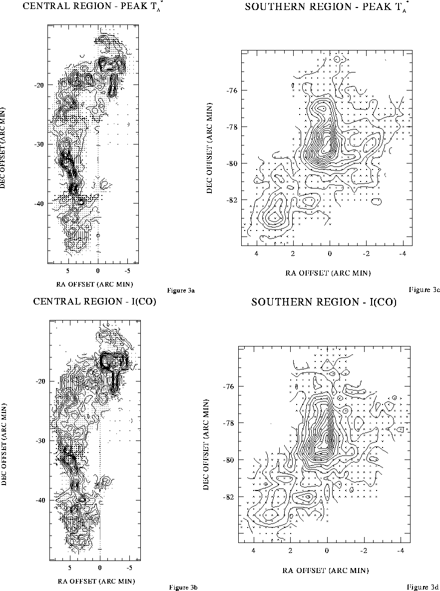
Figure 3: CO maps for the Central and Southern regions. In each
map, the dots show the locations of observations. (![]() ) offsets
are from the reference position,
) offsets
are from the reference position,
![]() ,
, ![]()
![]() 00' 00''. a) Peak
00' 00''. a) Peak ![]() for the Central region. Contour
levels are 0.3 to 3.9 in steps of 0.3 (where 0.3 is 3 times the rms noise
level). b) Peak
for the Central region. Contour
levels are 0.3 to 3.9 in steps of 0.3 (where 0.3 is 3 times the rms noise
level). b) Peak ![]() for the Southern region. Contour levels are
0.3 K to 3.9 K in steps of 0.3 K (where 0.3 K is 3 times the rms
noise level). c)
for the Southern region. Contour levels are
0.3 K to 3.9 K in steps of 0.3 K (where 0.3 K is 3 times the rms
noise level). c) ![]() for the Central region. Contour levels
are 1.0, 2.0, 4.0, 6.0, ..., 28.0 K km s
for the Central region. Contour levels
are 1.0, 2.0, 4.0, 6.0, ..., 28.0 K km s![]() . The velocity range for
the integration is 205 to 255 km s
. The velocity range for
the integration is 205 to 255 km s![]() . d)
. d) ![]() for the Southern
region. Contour levels are 1.0, 2.0, 4.0, 6.0, ..., 28.0 K km s
for the Southern
region. Contour levels are 1.0, 2.0, 4.0, 6.0, ..., 28.0 K km s![]() .
The velocity range for the integration is 205 to 270 km s
.
The velocity range for the integration is 205 to 270 km s![]()
In the Central region, we see a striking extended feature. It has
the appearance of being part of an arc, and is some 600 pc in
extent. Even in the integrated or peak intensity maps, it breaks
into a large number of CO concentrations. This type of structure
is similar to that seen in rich GMC complexes in the Milky Way,
e.g the Orion-Monoceros complex. In the Southern region, the
emission is not as extended, being only ![]() 150 pc in extent. One
peak is obvious, and there are other sub-peaks around. This is
similar to Milky Way complexes with a few GMCs.
150 pc in extent. One
peak is obvious, and there are other sub-peaks around. This is
similar to Milky Way complexes with a few GMCs.
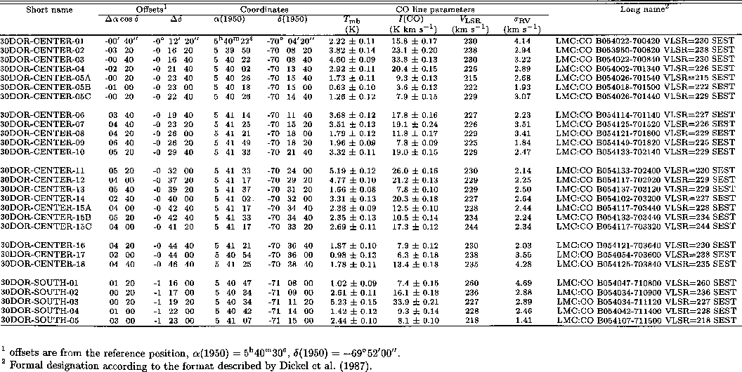
Table 1: Parameters of CO peaks in 30DOR Complex
To separate the emission into individual clouds, it is important
to isolate emission in individual velocity ranges. In the Milky
Way, the typical cloud-cloud velocity dispersion is about 5 to 6
km s![]() (Stark 1979), so it is convenient to use bins of
approximately that size. This is a convenient range for the LMC
also. Therefore, in Fig. 4 (click here), we present contours of
(Stark 1979), so it is convenient to use bins of
approximately that size. This is a convenient range for the LMC
also. Therefore, in Fig. 4 (click here), we present contours of ![]() integrated over successive velocity ranges, each 5.0 km s
integrated over successive velocity ranges, each 5.0 km s![]() wide.
In our efforts to isolate individual clouds, we prepared two set
of maps offset half of this step (2.5 km s
wide.
In our efforts to isolate individual clouds, we prepared two set
of maps offset half of this step (2.5 km s![]() ) from these maps, so we
would not miss emission at the edges of the integration ranges.
These have not been reproduced here, because the information they
contain overlaps with that in Fig. 4 (click here). For each region we show
maps over the velocity range for which significant emission is
seen. Note that for the Southern region there is no emission
between 240 and 255 km s
) from these maps, so we
would not miss emission at the edges of the integration ranges.
These have not been reproduced here, because the information they
contain overlaps with that in Fig. 4 (click here). For each region we show
maps over the velocity range for which significant emission is
seen. Note that for the Southern region there is no emission
between 240 and 255 km s![]() .
.
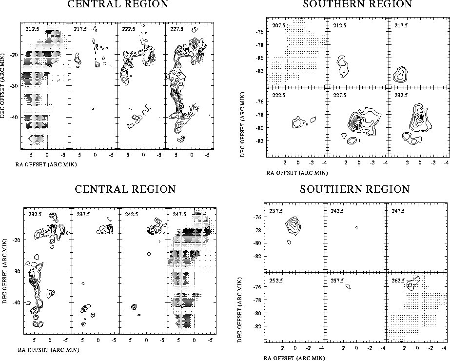
Figure 4: CO channel maps the Central and Southern regions. The
maps are integrated in 5 km s![]() steps covering the full range over
which significant emission is seen. The central velocity for the
5 km s
steps covering the full range over
which significant emission is seen. The central velocity for the
5 km s![]() range is shown on each panel. For each region, the dots
showing the locations of the observations are in the first and last maps
only. Contours are 1.0, 2.0, 4.0, 6.0, ..., 14.0 K km s
range is shown on each panel. For each region, the dots
showing the locations of the observations are in the first and last maps
only. Contours are 1.0, 2.0, 4.0, 6.0, ..., 14.0 K km s![]() for all
of the maps. (
for all
of the maps. (![]() ) offsets are from the reference position,
) offsets are from the reference position,
![]() ,
, ![]()
In the Central region, the channel maps show that the emission is coming from clouds that are localized in position and velocity. This is important since it shows that it is meaningful to talk about the CO emission as coming from clouds (possibly like those in the Milky Way), rather than having some extended uniform emission. In the Southern region, we see the emission breaking into cloud like structures. These channel maps have been used to identify individual molecular clouds. Some 22 clouds were found in the Central region and some 5 clouds were found in the Southern region. The identification of these clouds, and their large scale properties (sizes, velocity dispersions, CO luminosities and masses), will be discussed in Paper VII.
The basic observed properties of the clouds that we have
identified are shown in Table 1. In Col. 1 we give the cloud
name, in Cols. 2 and 3, we give the (![]() ) offsets from the
reference position
) offsets from the
reference position ![]() ,
, ![]() . In Cols. (4) and (5) we give the coordinates of the
peak. In Col. (6) we give the peak
. In Cols. (4) and (5) we give the coordinates of the
peak. In Col. (6) we give the peak ![]() , and in Col. (7) we give
, and in Col. (7) we give
![]() at the peak. In Col. (8), is the lsr velocity of the peak, in
Col. (9), we give the linewidth at the peak, expressed as a
dispersion,
at the peak. In Col. (8), is the lsr velocity of the peak, in
Col. (9), we give the linewidth at the peak, expressed as a
dispersion, ![]() . These are the formal temperature weighted
dispersions (rather than simply being the result of fitting). If
the line were a gaussian, then the full width a half maximum would
be 2.35
. These are the formal temperature weighted
dispersions (rather than simply being the result of fitting). If
the line were a gaussian, then the full width a half maximum would
be 2.35 ![]() .
.
The short names given in Table 1 recognize the division of the clouds into the Central and Southern complexes. Within those complexes the clouds are ordered, roughly, in order of their distance from 30Dor. Thus clouds with numbers near each other, also appear near each other in the sky. In addition to the short names given in Table 1, we have also assigned formal names to the clouds, according to the convention proposed by the IAU, as described by Dickel et al. (1987). These formal designations are also given in Table 1.
In order to look for systematic velocity structure, such as
rotation or expansion, it is useful to look at coordinate-velocity
maps. A selection of these maps is shown in Fig. 5 (click here). In Fig. 5 (click here)a
we see declination-velocity plots for the Central region. The first
is at an RA offset of -2.33'. This allows us to investigate the
velocity structure in the western extension of the cloud. There
is no strong pattern. Note that the emission that protrudes south
from the northwest corner of the arc, mostly associated with cloud
30Dor Central 04, is at a ![]() of about 240 km s
of about 240 km s![]() , while the rest
the emission from the northern part of the arc is at 225 km s
, while the rest
the emission from the northern part of the arc is at 225 km s![]() .
This suggests that the protruding cloud is kinematically distinct
from the rest of the arc. The next
.
This suggests that the protruding cloud is kinematically distinct
from the rest of the arc. The next ![]() plot is at an RA offset of
+4', which brings it through the longest part of the cloud. There
is very little velocity structure at the top and bottom, except
for the presence of a second source at DEC offset -41', at 245
km s
plot is at an RA offset of
+4', which brings it through the longest part of the cloud. There
is very little velocity structure at the top and bottom, except
for the presence of a second source at DEC offset -41', at 245
km s![]() . In the center of the main part of the emission, there is a
trend of higher velocities as one goes farther north (the same
sense as the gradient in the Southern region). This shows up more
clearly in the next frame, which shows a
. In the center of the main part of the emission, there is a
trend of higher velocities as one goes farther north (the same
sense as the gradient in the Southern region). This shows up more
clearly in the next frame, which shows a ![]() plot at RA offset of
+5', where the emission from the Central region is stronger. The
gradient along there is 0.9 km s
plot at RA offset of
+5', where the emission from the Central region is stronger. The
gradient along there is 0.9 km s![]() arcmin
arcmin![]() or 0.06 km s
or 0.06 km s![]() pc
pc![]() .
We have also looked at a number of right-ascension-velocity plots at
various declinations, and no obvious patterns are seen. These are
not presented here.
.
We have also looked at a number of right-ascension-velocity plots at
various declinations, and no obvious patterns are seen. These are
not presented here.
In Fig. 5 (click here)b we present coordinate-velocity plots for the Southern
region. The lower panel, which shows a ![]() diagram, exhibits
two clear peaks, one at 228 km s
diagram, exhibits
two clear peaks, one at 228 km s![]() , and the other at 236 km s
, and the other at 236 km s![]() . In
comparing this with the
. In
comparing this with the ![]() for the same region, only the
stronger peak is visible, while the weaker one is simply lost in
the broader emission. With the coordinate velocity map, we can
see that these are two distinct peaks. The smooth connection
between the two could result from the overlap of the emission from
two distinct clouds, or it could be a real connection, with the
velocity shift arising from cloud rotation, with the upper part of
the complex moving away from us. This would correspond to a
velocity gradient of 3.5 km s
for the same region, only the
stronger peak is visible, while the weaker one is simply lost in
the broader emission. With the coordinate velocity map, we can
see that these are two distinct peaks. The smooth connection
between the two could result from the overlap of the emission from
two distinct clouds, or it could be a real connection, with the
velocity shift arising from cloud rotation, with the upper part of
the complex moving away from us. This would correspond to a
velocity gradient of 3.5 km s![]() arcmin
arcmin![]() , or 0.2 km s
, or 0.2 km s![]() pc
pc![]() .
In the upper frame, showing an
.
In the upper frame, showing an ![]() diagram, we again see
two distinct peaks, but only a small velocity shift or gradient.
diagram, we again see
two distinct peaks, but only a small velocity shift or gradient.
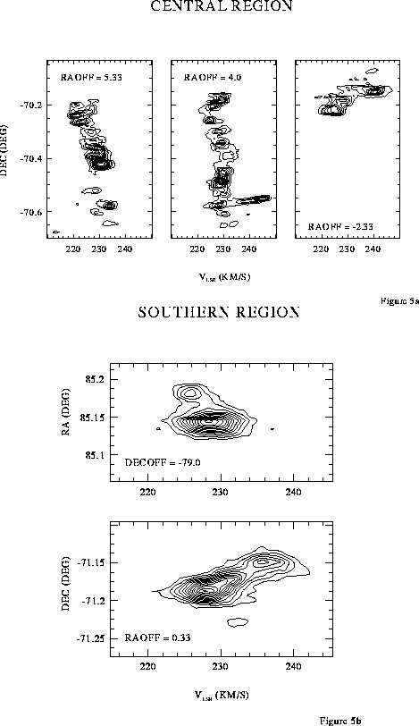
Figure 5: Selected coordinate velocity maps for the Central region
and for the Southern region. (![]() ) offsets are from the
reference position,
) offsets are from the
reference position, ![]() ,
,
![]()