In some instances the cyclic nature of the FT + inversion process may render it unsuitable. The most intractable cases are those for which something happens at the scan ends which is different in physical process from that governing the general run of the scan. It may be that an undesirable amount of high-frequency component is needed in the filter to fit the extremeties, leaving the center of the baseline fluctuating too violently. Judicious pruning of scan-ends (which may contain suspect data anyway) may solve the problem.
But what about buried lines or faint broad lines? Or just plain faint lines which have not been patched? It is fair criticism that such line amplitudes will be reduced because the unseen signal was not ``patched out", and the filter process has indeed removed some of the low-frequency components which would have contributed to their amplitudes. However, no objective technique is going to correct for unseen features; and if features are strong enough to recognize or sense, they are strong enough to patch. Concern about the signal reduction which results in not patching very weak lines, signal which is statistically known, can be assessed by Monte-Carlo analysis (e.g. Wall et al. 1982).
Techniques of polynomial or spline fits, or of heavy smoothing, are generally less objective than Fourier analysis. They do not avoid the signal-reduction difficulty, and in each of these cases, some form of ``patching" and treatment of the scan ends is going to be required.
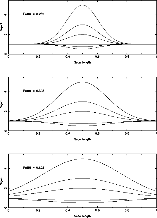
Figure 5: Part of the set of distorted continua on which
signals are placed to carry
out the error analysis. Each continuum of unit length consists of a
Gaussian of height b added at the mid-point of a base of unity.
The 5 values of b are 4.0, 2.0, 1.0, -.25 and -.50. The calculations
were carried out with 6 families of these baselines, the Gaussians
having half-widths of 0.250, 0.395, 0.628, 0.995, 1.577 and 2.500
scan-lengths. The first three of these are shown above
It is difficult to make a comparative error analysis; the numerous and ill-disciplined ways in which baselines or continua are normally derived do not provide standard models against which comparison can be made. One of the advantages of the technique described above is to enable a formal estimate of the error in signal and/or equivalent width which results from continuum assessment.
The minimum-component technique results in
perfect fits and perfect flux measurement (except for noise)
if the baseline is linear. It is only when signal sits on bumps or in
hollows that error results.
To carry out an analysis of such errors,
a simple model of a continuum and a signal
based on Gaussians was adopted. The geometry, shown in Fig. 5 (click here) and
Fig. 6 (click here),
consists of Gaussian signals of ![]() sitting at the maxima or minima
of continua built of a unit dc level plus a centered
Gaussian of height
b and given FWHM. The data stream is of unit length and the Gaussian
signal is
of height h(b+1), i.e. h is the ratio of the signal height to the
centrepoint of the continuum.
sitting at the maxima or minima
of continua built of a unit dc level plus a centered
Gaussian of height
b and given FWHM. The data stream is of unit length and the Gaussian
signal is
of height h(b+1), i.e. h is the ratio of the signal height to the
centrepoint of the continuum.
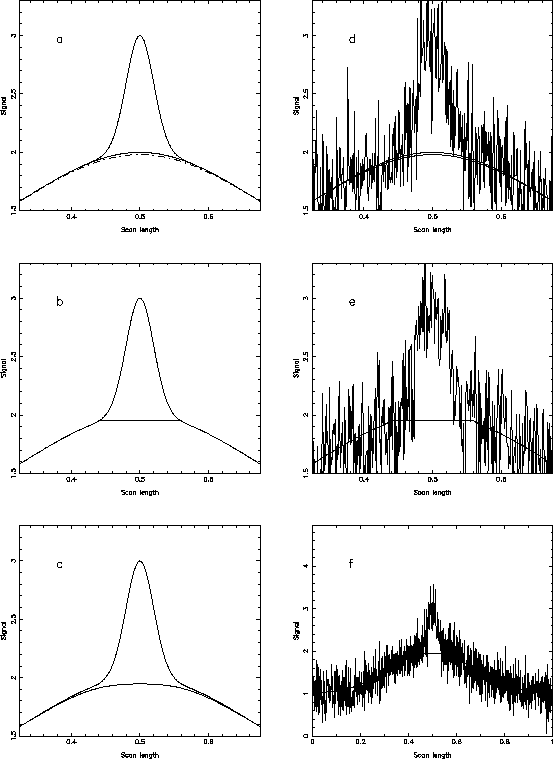
Figure 6: Panel a) shows a Gaussian signal of ![]() sitting at the maximum of the member of the distorted-continuum family
of Fig. 5 with b= 1.0, FWHM = 0.395. The true
baseline is the solid curve and the minimum-component baseline selected to
give a 1% error is the dash-dot curve. The signal amplitude
sitting at the maximum of the member of the distorted-continuum family
of Fig. 5 with b= 1.0, FWHM = 0.395. The true
baseline is the solid curve and the minimum-component baseline selected to
give a 1% error is the dash-dot curve. The signal amplitude ![]() . Panel b) shows the total curve
with a patch at
. Panel b) shows the total curve
with a patch at ![]() , while panel c) is the resultant
baseline after filtering the patched curve of b) by limiting the
Fourier components in the reconstruction
of the patched approximation as described. Panels
d) and e) are panels a) and b) with noise of rms =
0.15h added for verisimilitude, while panel f) shows the entire
scan length with the minimum-component continuum. In this example the
error in
equivalent width with the minimum-component baseline is 13%; if
, while panel c) is the resultant
baseline after filtering the patched curve of b) by limiting the
Fourier components in the reconstruction
of the patched approximation as described. Panels
d) and e) are panels a) and b) with noise of rms =
0.15h added for verisimilitude, while panel f) shows the entire
scan length with the minimum-component continuum. In this example the
error in
equivalent width with the minimum-component baseline is 13%; if ![]() is doubled
at 0.02, this error rises to 50%
is doubled
at 0.02, this error rises to 50%
In this (or any) model of the continuum the sources of error in signal measurement are the following.
In the current methodology, it is possible that the baseline may be badly fit by not allowing enough Fourier components to take part in the assembly of the filtered baseline - we are trying to use the minimum number of components in order to produce the best approximation and to avoid including any noise or signal. The difficulty as illustrated in Fig. 6 (click here) may be that in the presence of noise, this badness of the fit goes unrecognized.
Note that if equivalent width is calculated, it exacerbates the errors, in the sense that the flux error due to the baseline error increases the measured equivalent width over the true, while the baseline error itself decreases the baseline and thus also increases the measured equivalent width over the true.
Even with the simplistic model of Fig. 5 (click here) and Fig. 6 (click here), there is a large parameter space. The estimates carried out here are representative only, but provide a guide from which to determine approximate errors in most such analyses. To restrict the parameter space, two assumptions were made:
Measured and true equivalent widths were calculated for Gaussian signals centered on baselines in the family of Fig. 5 (click here). This may be done analytically because of the additive nature of Fourier transforms. For the patched/filtered scan, the transform of two truncated Gaussians (regions A and C) separated by a rectangular region (B, corresponding to the patch), can be multiplied by the filter function
![]()
to obtain the signal error after reverse transformation, as
![]()
where ![]() is the true flux and the signal flux is measured out to
is the true flux and the signal flux is measured out to
![]() about its centroid.
about its centroid.
In practice it was simplest to use the FT system set up to analyze the real data (Laing et al. 1994 and in preparation). Checking such calculations is simple because there are at least three cases where geometrical analysis gives close approximation. Consider the following two examples.
![]()
In this case the error on the baseline due to
filtering (inclusion of too few components) dominates. Suppose this
error is ![]() . Then the ratio of measured to true equivalent
width is
. Then the ratio of measured to true equivalent
width is
![]()
where the flux is summed over ![]() about the signal centre.
about the signal centre.
for measurement over ![]() .
The last two terms represent the area in the top of the Gaussian distortion
which is included by virtue of the patch at
.
The last two terms represent the area in the top of the Gaussian distortion
which is included by virtue of the patch at ![]() .
.
The measured equivalent width becomes
![]()
Figure 7: Ratio of measured equivalent width to true equivalent width against
![]() , the signal dispersion in units of scan length,
for a Gaussian signal sitting at the peak of a continuum whose Gaussian
FWHM = 0.628 and b = 1.0. The baseline has been estimated as described in
the text, using a filter width to produce (in the absence of signal)
a 1% deviation of the filtered baseline from the true baseline. The
patch width and the width over which the flux is measured is
, the signal dispersion in units of scan length,
for a Gaussian signal sitting at the peak of a continuum whose Gaussian
FWHM = 0.628 and b = 1.0. The baseline has been estimated as described in
the text, using a filter width to produce (in the absence of signal)
a 1% deviation of the filtered baseline from the true baseline. The
patch width and the width over which the flux is measured is
![]() . The height of the signal Gaussian is h(b+1), and the
curves are computed for different signal strengths with values of h as
shown
. The height of the signal Gaussian is h(b+1), and the
curves are computed for different signal strengths with values of h as
shown
The computed results (with which these approximations agree)
are shown in Fig. 7 (click here) to Fig. 11 (click here). In
Fig. 7 (click here), the error dependence
on width of signal is shown for a given member of the continuum family
in Fig. 5 (click here).
For small and narrow signals, the error is almost totally due to
the 1% baseline
deviation. The error drops slightly as signal width increases,
the total flux of the signal dominating the extra signal. But as signal
width increases further, the error rises rapidly as the patching process
includes some of the peak of the Gaussian scan distortion in the total
flux estimation. For strong signals the situation is completely
different; at small ![]() the estimate is accurate as the 1% baseline
error is negligible. But as
the estimate is accurate as the 1% baseline
error is negligible. But as ![]() increases, the ratio drops below unity
because the
increases, the ratio drops below unity
because the ![]() patch is not at the base of the signal; the
excess signal now pulls up the (relatively weak) baseline, and this
overestimate of the baseline dominates the error in measured
equivalent width. Hence for very strong sources, as
patch is not at the base of the signal; the
excess signal now pulls up the (relatively weak) baseline, and this
overestimate of the baseline dominates the error in measured
equivalent width. Hence for very strong sources, as ![]() increases,
the equivalent width becomes progressively underestimated.
These effects are in general identifiable, depending on the
signal-to-noise ratio (Fig. 6 (click here)).
increases,
the equivalent width becomes progressively underestimated.
These effects are in general identifiable, depending on the
signal-to-noise ratio (Fig. 6 (click here)).
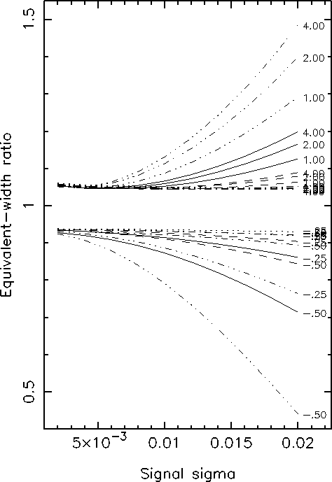
Figure 8: Ratio of measured to true equivalent width versus
width of signal in units
of scan-length. The height parameter of the Gaussian signal
(total height = h(b+1)) is fixed at h=0.5, and the patch
width is fixed at ![]() . The scale-length
of the Gaussian
distortion on the unit dc baseline is varied: FWHM = 0.25 scan-length,
triple-dot - dash lines; FWHM = 0.395, solid lines; FWHM = 0.628,
dashed lines; FWHM = 0.995, dot-dash lines; and FWHM = 1.577 dotted lines.
The amplitude of the distortion is varied, with b taking five values,
-.25, -.5, 1.0, 2.0 and 4.0, marked against the curves. There is
a small asymmetry of 0.5% about the value of 1.0, a second-order effect
due to the patch pulling the filtered baseline towards it
. The scale-length
of the Gaussian
distortion on the unit dc baseline is varied: FWHM = 0.25 scan-length,
triple-dot - dash lines; FWHM = 0.395, solid lines; FWHM = 0.628,
dashed lines; FWHM = 0.995, dot-dash lines; and FWHM = 1.577 dotted lines.
The amplitude of the distortion is varied, with b taking five values,
-.25, -.5, 1.0, 2.0 and 4.0, marked against the curves. There is
a small asymmetry of 0.5% about the value of 1.0, a second-order effect
due to the patch pulling the filtered baseline towards it
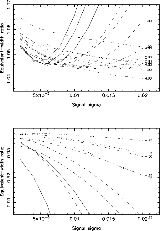
Figure 9: As for Fig. 8, except that the vertical scale is much expanded
to show what happens for the continua of lesser distortion. The curves
are for Gaussian distortions on unit baselines of FWHM = 0.395 scan length,
solid lines;
FWHM = 0.628, dashed lines; FWHM = 0.995, dot-dash lines; FWHM = 1.577,
dotted lines; and FWHM = 2.50, triple-dot - dash lines
In Fig. 8 (click here), a fixed value of h, signal height, was adopted, and the error is shown again as a function of signal width. Here the effects of the different distortions of baseline are shown, i.e. a representative set of the continuum family of Fig. 5 (click here) is introduced. The central gap is the effect of the 1% baseline fit; for a convex scan (positive b) it is to overestimate the equivalent width, while for a concave scan (negative b), it is to underestimate. For smaller scale-length and for the larger b values, the measured equivalent width deviates rapidly from the true value because of error in continuum estimate and (more important) the inclusion of baseline in the signal estimate. These effects diminish with decreasing b and with increased FWHM. The error is drastically less for members of the family which curve gently, and Fig. 9 (click here) shows scales expanded about the central gap to illustrate the dependence of errors in these situations.
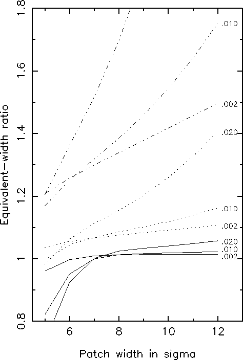
Figure 10: Ratio of measured equivalent width to true equivalent width as a
function of patch width. The Gaussian signal, of standard deviation
![]() , 0.01 or 0.02 as marked,
is positioned at the crest of the distorted baseline with b=1.0 and
FWHM = 0.628. The dot-dash curves are for signal height h=0.1, the
dotted curves for h=0.5, and the solid curves for h=10.0. The minimum
components have been chosen to give a 1% maximum baseline error
, 0.01 or 0.02 as marked,
is positioned at the crest of the distorted baseline with b=1.0 and
FWHM = 0.628. The dot-dash curves are for signal height h=0.1, the
dotted curves for h=0.5, and the solid curves for h=10.0. The minimum
components have been chosen to give a 1% maximum baseline error
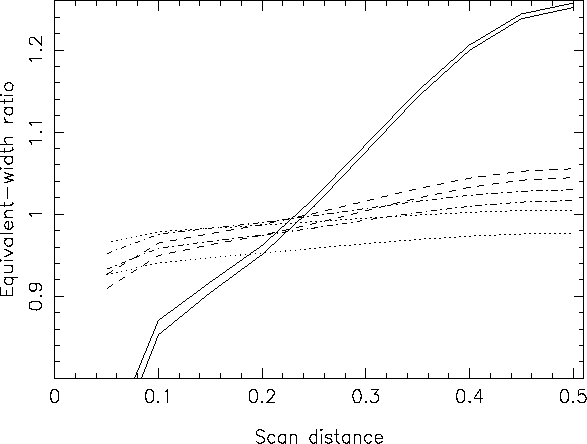
Figure 11: Ratio of measured equivalent width to true equivalent width as a
function of distance along scan. Previous error curves have all been
computed with the signal centered at the max/min of the baseline. Here the
Gaussian signal is moved along the scan from the edge to the centre (at 0.5).
The single continuum model adopted has a Gaussian of height b = 1.0,
FWHM = 0.628 sitting on a dc level of 1.0. The
curves shown are for Gaussian signals of h = 0.1 (solid lines),
0.5 (dashed lines), 1.0 (dash-dot lines), and 5.0 (dotted lines). Patch width
and flux measurement is over ![]() in each case. The two lines for
each signal height are for
in each case. The two lines for
each signal height are for ![]() (upper) and 0.01. The minimum
components have been chosen to give a 1% maximum baseline error
(upper) and 0.01. The minimum
components have been chosen to give a 1% maximum baseline error
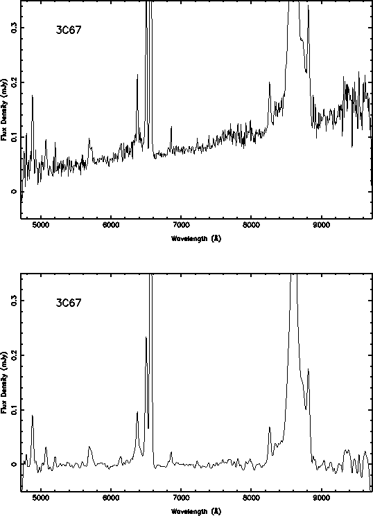
Figure 12:
The spectrum of 3C 67 (Laing et al. 1994) to which bandpass
filtering has been applied. The lower panel shows the
results of removing low-frequency components, i.e. the continuum, by
the process described above, and by removing the highest-frequency
components to improve signal-to-noise ratio
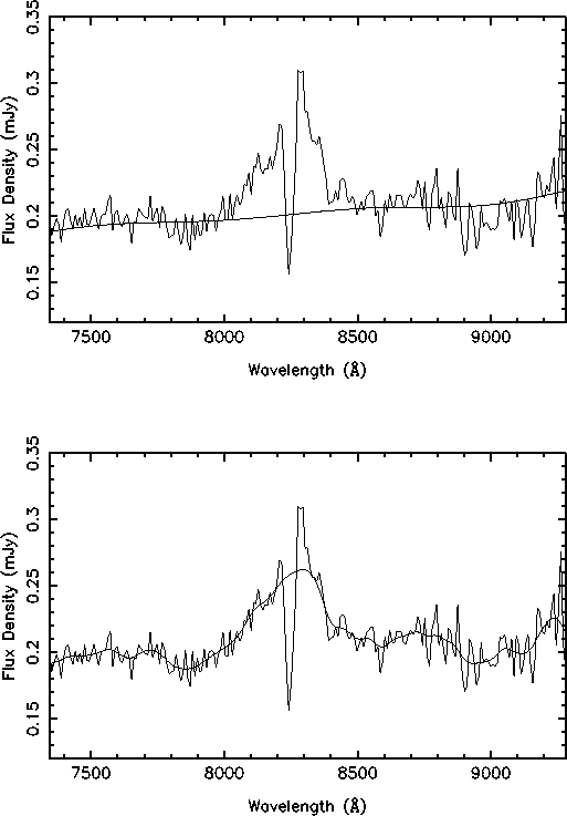
Figure 13:
A portion of the optical spectrum of 3C 191 showing the
broad emission line of MgII at ![]() 2800 Å (rest frame),
cut by a narrow absorption line. The upper panel shows the emission line
together with a baseline determined as for 3C 47; the lower
panel shows a ``baseline" in which
2800 Å (rest frame),
cut by a narrow absorption line. The upper panel shows the emission line
together with a baseline determined as for 3C 47; the lower
panel shows a ``baseline" in which ![]() (rather than
(rather than
![]() ) was used in the Gaussian taper, constructing a ``baseline"
from many more low-frequency components. From these two ``continuum" estimates,
parameters (equivalent width, etc.) of both the absorption and
the emission line could be measured
) was used in the Gaussian taper, constructing a ``baseline"
from many more low-frequency components. From these two ``continuum" estimates,
parameters (equivalent width, etc.) of both the absorption and
the emission line could be measured
![]()
Figure 14:
The spectrum of 3C48, with baseline assessment
by a fully objective procedure. The smooth lines show baseline
iterations: 1 - dotted; 2 - dot-dash; 20 - dashed; 150 - full
Figure 10 (click here) illustrates the effect of varying the patch width.
For the weaker
sources (h=0.1 and 0.5) the equivalent width is consistently
overestimated for convex baselines. The overestimate increasing dramatically
and monotonically with patch width because the patch lowers the
effective continuum used to estimate the equivalent width while increasing
the amount of continuum erroneously included in measurement of signal.
For strong sources the ratio becomes insensitive to patch width as the
continuum appears almost flat to the source. The dominant effect is for
short patches; as the width shrinks below ![]() , signal
is underestimated while the patch becomes placed relatively
high into the signal, raising the estimated continuum significantly
with respect to the true continuum. Both effects reduce the
measured equivalent width.
, signal
is underestimated while the patch becomes placed relatively
high into the signal, raising the estimated continuum significantly
with respect to the true continuum. Both effects reduce the
measured equivalent width.
The following points emerge from the error analysis.
Two things must be borne in mind when using the present results
to estimate errors on equivalent widths.
Firstly, the worst-case situation has been examined in which the signal
sits at the point of maximum inflection, at the centre of the continuum
models. Figure 11 (click here) shows that for the Gaussian model continua
on average the magnitude of the errors is about half these maximum values,
the error on the ![]() linear flanks of the Gaussian being close to zero.
Secondly, the curves have been
computed on the basis of ``1%" continuum fits. These too are pessimistic;
experience shows that the minimum-component
baselines are generally more accurate than this.
linear flanks of the Gaussian being close to zero.
Secondly, the curves have been
computed on the basis of ``1%" continuum fits. These too are pessimistic;
experience shows that the minimum-component
baselines are generally more accurate than this.
The analysis indicates how rapidly errors in equivalent widths can escalate with non-linear continua, even when the procedures for continuum assessment and signal measurement are well defined. When yet broader wings are involved, the errors produced will be substantially greater. The analysis goes some way to explaining why estimates of line-fluxes in the literature can differ by a factor of two, even with reasonable signal-to-noise.
Harmonic analysis for scans (data-series) is powerful and versatile. Having assessed the harmonic content via an FT, formal techniques can be developed on the basis e.g. of known instrumental parameters to apply low and high-frequency filtering automatically to the data both to remove (or assess) the continuum and to improve signal-to-noise ratio. This is bandpass filtering, and an example is shown in Fig. 12 (click here). And indeed there are further uses of the methodology, Fig. 13 (click here) showing as an example the evaluation of the equivalent width of an absorption line in the midst of a strong emission line.
In addition the technique advocated here may be automated if some assumptions
about the signal are made. For instance, if all signals are
unresolved, an iterative procedure may be developed using differences
between first approximations to a baseline and the
original data to decide upon regions to patch; patch widths are then
simply the instrumental resolution width. A second iteration is then
carried out with the new baseline to decide if additional regions
need patching. For the more general case in which the signal is resolved,
different algorithms may be appropriate. Figure 14 (click here) shows
an example.
As before, a ``baseline array"
is formed from which a baseline is constructed from the few
lowest-spatial-frequency components.
In the first instance,
the baseline array is set as the data array, and the first iteration
consists of forming a baseline from the lowest-spatial-frequency
components. Each subsequent iteration consists of
finding the largest difference between the previous baseline and the data
array, and then replacing the data in the baseline array
with the data from the previous baseline iteration,
and ![]() half-width of the instrument profile about this point.
A different region of replacement was demanded for
all subsequent iterations. The algorithm is very inefficient, but effective
for virtually all the spectra tried so far, with the exception of spectra for
which very strong broad emission/absorption lines occur at the ends of the
scans. But almost all procedures struggle under this circumstance.
Many different algorithms could be adopted to improve efficiency: broader
patches, a line-list as a starting point,
etc. There is resemblance in such procedures to
the CLEAN technique (Högbom 1974) used in radio astronomy
synthesis mapping.
half-width of the instrument profile about this point.
A different region of replacement was demanded for
all subsequent iterations. The algorithm is very inefficient, but effective
for virtually all the spectra tried so far, with the exception of spectra for
which very strong broad emission/absorption lines occur at the ends of the
scans. But almost all procedures struggle under this circumstance.
Many different algorithms could be adopted to improve efficiency: broader
patches, a line-list as a starting point,
etc. There is resemblance in such procedures to
the CLEAN technique (Högbom 1974) used in radio astronomy
synthesis mapping.
Acknowledgements
I am grateful to Robert Laing, Charles Jenkins and Steve Unger for permission to use data before publication, and to Pierre Maxted for supplying me with the digitized version of the observation of RZ Cas. I appreciated helpful comments on drafts by David Carter, Charles Jenkins and a referee.