In addition to the HG-analysis presented here we have
made exactly the same analysis for the 1984 to 1989 Carlsberg data.
Combining the two data sets we get a 10-year coverage for some
asteroids. This gives quite good statistics on how the
phase curves change with opposition longitude.
For asteroids with a known spin vector direction we can further
compute the aspect angle of the observations.
In this paper we define the aspect angle ![]() as the angle between the
asteroid spin vector and the reverse of the phase angle bisector (PAB).
Spin vectors were taken from the collection of spin vector determinations
by Magnusson et al. (1994).
We used the first synthesis solution for each asteroid.
Aspect angles for 23 of our current sample of asteroids were
obtained in this way.
We have looked at graphs of the dependence of H and G on the
aspect angle
as the angle between the
asteroid spin vector and the reverse of the phase angle bisector (PAB).
Spin vectors were taken from the collection of spin vector determinations
by Magnusson et al. (1994).
We used the first synthesis solution for each asteroid.
Aspect angles for 23 of our current sample of asteroids were
obtained in this way.
We have looked at graphs of the dependence of H and G on the
aspect angle ![]() for all these objects.
Examples of the H-dependence are shown in Fig. 3 (click here).
for all these objects.
Examples of the H-dependence are shown in Fig. 3 (click here).
For objective analysis of these graphs we fit 2nd order Legendre series:

Light scattering is probably closest to the geometric approximation at zero
solar phase. Therefore the modeled reduced magnitude H at ![]() is usually used.
However, in practice this value is obtained from extrapolation from observed
solar phases, and thus sensitive to errors in the slope parameter G.
In order to reduce this source of error we instead use the model magnitude
at
is usually used.
However, in practice this value is obtained from extrapolation from observed
solar phases, and thus sensitive to errors in the slope parameter G.
In order to reduce this source of error we instead use the model magnitude
at ![]() , which is near the mean observed solar phase angle.
, which is near the mean observed solar phase angle.
![]()
Figure 3: Two good examples of the aspect dependence of the slope parameter H.
Both show a ``U-shaped'' pattern typical of bodies with polar flattening.
The values above the diagrams are ecliptic coordinates of the spin vector used
For most asteroids there are two symmetric spin vector solutions
that both fit the observations equally well.
If the second synthesis solution in Magnusson (1996)
is choosen instead of the first one then approximately the same
coefficients results, except that ![]() and
and ![]() have opposite sign.
have opposite sign.
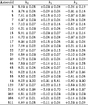
The Legendre coefficients for 23 asteroids are presented in Table 3 (click here).
The tabulated error estimates are based on the quality of fit.
The variations in ![]() are probably due to changing geometrical cross-sections,
and, to lesser extent, differences in average albedo at different
latitudes on the asteroid surfaces.
Non-zero coefficients
are probably due to changing geometrical cross-sections,
and, to lesser extent, differences in average albedo at different
latitudes on the asteroid surfaces.
Non-zero coefficients ![]() are most naturally interpreted
as differences in albedo on the northern and southern hemispheres.
The second Legendre component is probably due mostly to polar flattening,
as evident from the clear dominance of negative
are most naturally interpreted
as differences in albedo on the northern and southern hemispheres.
The second Legendre component is probably due mostly to polar flattening,
as evident from the clear dominance of negative ![]() -values in Table 3 (click here).
However, differences in albedo between equatorial and polar regions
may also contribute to
-values in Table 3 (click here).
However, differences in albedo between equatorial and polar regions
may also contribute to ![]() .
.

Table 3: A summary of the Legendre coefficients
The Legendre coefficients are a natural way of descibing the light
scattering, but most asteroid shape models take the form of tri-axial
ellipsoids with axis-ratios ![]() (Magnusson et al. 1989).
These models are often based on extensive lightcurve photometry,
with lightcurve amplitudes giving quite reliable ratios a/b.
However, the b/c-ratios are often ill-defined because amplitudes
give very model-dependent b/c-values and the absolute calibration
of lightcurve photometry are often heterogenous.
The Carlberg data have the opposite characteristics,
i.e. homogenous absolute calibration and bad lightcurves,
and they therefore complement standard photometry well.
We therefore use a/b-ratios from other models as input,
and compute b/c-ratios from the Carlsberg data.
(Magnusson et al. 1989).
These models are often based on extensive lightcurve photometry,
with lightcurve amplitudes giving quite reliable ratios a/b.
However, the b/c-ratios are often ill-defined because amplitudes
give very model-dependent b/c-values and the absolute calibration
of lightcurve photometry are often heterogenous.
The Carlberg data have the opposite characteristics,
i.e. homogenous absolute calibration and bad lightcurves,
and they therefore complement standard photometry well.
We therefore use a/b-ratios from other models as input,
and compute b/c-ratios from the Carlsberg data.
The difference between the mean polar H-value and the equatorial H-value
is ![]() .
By equating the corresponding brightness ratio,
.
By equating the corresponding brightness ratio, ![]() ,
with the ratio between the area of the projection of the model along the spin axis,
,
with the ratio between the area of the projection of the model along the spin axis, ![]() ,
and the mean perpendicular cross-section,
,
and the mean perpendicular cross-section, ![]() ,
and solving for b/c, we obtain the approximate relation:
,
and solving for b/c, we obtain the approximate relation:
![]()
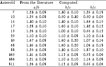
Table 4 (click here) shows the axes ratios for the best cases where the errors are not too high. The accuracy seems to be similar to the dispersion of b/c-values from ordinary photometry (Magnusson, in preparation). The number of apparitions is so low that a single bad phase curve can easily ruin the Legendre fit.

Table 4: Ellipsoidal model axis ratios
For most of the objects
no significant variation of G-values were found to indicate
any clear aspect dependence. In general the estimated errors
in ![]() and
and ![]() are of the same order as the values
themselves. We find, however, some indication of different G-values
between the northern and southern hemispheres for the cases of (7) Iris and
(16) Psyche, but this has to be confirmed by further observations.
The latter case may confirm the finding by Lupishko & Belskaya (1983)
and
Lupishko et al. (1983) that (16) Psyche is among the objects that
have different albedos on the hemispheres.
are of the same order as the values
themselves. We find, however, some indication of different G-values
between the northern and southern hemispheres for the cases of (7) Iris and
(16) Psyche, but this has to be confirmed by further observations.
The latter case may confirm the finding by Lupishko & Belskaya (1983)
and
Lupishko et al. (1983) that (16) Psyche is among the objects that
have different albedos on the hemispheres.
In general the variations in G are probably associated with
surface variegation, different compositional and
morphological surface areas, and global shape effects.
However, we are perplexed by the clear dominance of negative ![]() -values,
which is opposite to our expectations.
To see why, let us consider equatorial lightcurves.
These generally show a clear increase in lightcurve amplitude
as the solar phase angle increases.
Within the framework of tri-axial models, with semi-axes
-values,
which is opposite to our expectations.
To see why, let us consider equatorial lightcurves.
These generally show a clear increase in lightcurve amplitude
as the solar phase angle increases.
Within the framework of tri-axial models, with semi-axes ![]() ,
this implies that the G-value measured along the a-axis
(looking down at the point of highest curvature)
is smaller than the G-value measured along the b-axis.
We expected a continuation of this trend with even larger G-values
when observing along the c-axis, which show the flat polar regions
with the lowest curvature in the model.
The result would have been positive
,
this implies that the G-value measured along the a-axis
(looking down at the point of highest curvature)
is smaller than the G-value measured along the b-axis.
We expected a continuation of this trend with even larger G-values
when observing along the c-axis, which show the flat polar regions
with the lowest curvature in the model.
The result would have been positive ![]() -values.
-values.