Before beginning the data reduction process it is important to ensure that
all recorded signals are synchronized with an accuracy better than one
sample interval ![]() . This might not be true if for example the
interferometric and photometric signals are delayed by different
electronics (e.g., analog filters) before being digitized and recorded. In
that case, the amount of desynchronization can be evaluated by looking at
the position of the correlation peak between I and the best linear fit to
I of
. This might not be true if for example the
interferometric and photometric signals are delayed by different
electronics (e.g., analog filters) before being digitized and recorded. In
that case, the amount of desynchronization can be evaluated by looking at
the position of the correlation peak between I and the best linear fit to
I of ![]() and
and ![]() . A corresponding offset is then applied to the
relevant signals; this leaves a few samples at the beginning or the end of
the sequence as undefined.
. A corresponding offset is then applied to the
relevant signals; this leaves a few samples at the beginning or the end of
the sequence as undefined.
An apodization of the corrected interferometric signal is necessary for several reasons: it solves the problem of undefined samples for the signals that have been synchronized, and it removes potential boundary effects when Fast Fourier Transforms (FFTs) are performed. Because it reduces the effective length of the sequence, apodization also contributes to attenuate the detector and piston noises.
Therefore before measuring ![]() , the signal
, the signal ![]() is multiplied by an apodization window A(x). Any smoothly
varying function could be employed; the following function was chosen
(assuming the OPD scan spans the interval
is multiplied by an apodization window A(x). Any smoothly
varying function could be employed; the following function was chosen
(assuming the OPD scan spans the interval ![]() ):
):

Thus the window blocks out the signal for ![]() , and provides a smooth transition to full transmission for
, and provides a smooth transition to full transmission for ![]() . The choice of
. The choice of
![]() and
and ![]() is not critical and depends essentially on the number of
fringes that can be seen above the noise level of the interferometric
detector. In the
is not critical and depends essentially on the number of
fringes that can be seen above the noise level of the interferometric
detector. In the ![]() Boo example, the signal is blocked out for
Boo example, the signal is blocked out for
![]() on each side of the scans, and the length of the transition
regions is
on each side of the scans, and the length of the transition
regions is ![]() .
.
For each photometric signal, the corresponding optimal filter is estimated
by using the power spectrum of the background current sequence as an
estimator ![]() of the
noise power spectral density. It is expected that the value of
of the
noise power spectral density. It is expected that the value of
![]() is close to 1 for low frequencies where the photometric
signal is strong, and decreasing to zero at higher frequencies where
detector noise dominates.
is close to 1 for low frequencies where the photometric
signal is strong, and decreasing to zero at higher frequencies where
detector noise dominates.
A problem arises at some higher frequencies when, because of statistical
fluctuations in the noise power density, the estimated noise power
![]() is smaller than
the measured signal power
is smaller than
the measured signal power ![]() .
This would imply a negative value for the Wiener filter. To avoid this, the
estimated Wiener filter is defined as such:
.
This would imply a negative value for the Wiener filter. To avoid this, the
estimated Wiener filter is defined as such:

where ![]() is the smallest wave number that meets the condition
is the smallest wave number that meets the condition
![]() . The value of
. The value of
![]() is forced to 1 at the continuum to maintain the
average value of the photometric signal.
is forced to 1 at the continuum to maintain the
average value of the photometric signal.
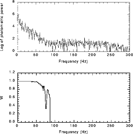
Figure 8: Spectral power of a photometric signal (top, note the logarithmic
scale) and its associated Wiener filter (bottom)
Figure 8 (click here) shows an example of photometric power density
and the associated ![]() .
.
Here is a link from the continuous world of functions to the discrete world
of computer data. The physical signal M(x) is sampled every ![]() and recorded in the computer as a series of numbers
and recorded in the computer as a series of numbers ![]() (
(![]() ) such that:
) such that:
![]()
Data reduction is performed by the computer on the ![]() series. The
continuous Fourier transform is replaced by a Fast Fourier Transform, which
produces a new series of N numbers (harmonics) Y
series. The
continuous Fourier transform is replaced by a Fast Fourier Transform, which
produces a new series of N numbers (harmonics) Y![]() . Positive
frequencies are represented by harmonics Y
. Positive
frequencies are represented by harmonics Y![]() to Y
to Y![]() (with Y
(with Y![]() being the Nyquist harmonic). If the physical signal
was correctly sampled (i.e. if
being the Nyquist harmonic). If the physical signal
was correctly sampled (i.e. if ![]() for
for ![]() ), then each Y
), then each Y![]() (
(![]() ) is linked to
) is linked to
![]() by the relationship
(Brigham 1974):
by the relationship
(Brigham 1974): ![]()
Therefore the numerical data reduction process yields a final series Z![]() of
complex numbers whose moduli for
of
complex numbers whose moduli for ![]() are linked to
are linked to ![]() by:
by:
![]()
The integral ![]() of the squared modulus of
of the squared modulus of ![]() can be evaluated numerically
using the trapezoidal rule:
can be evaluated numerically
using the trapezoidal rule:

It follows that the numerical value of ![]() can be computed from the
can be computed from the ![]() series with:
series with:

The numerical evaluation of ![]() is performed in a similar way.
is performed in a similar way.
In principle, to minimize the statistical fluctuations of ![]() the
integration boundaries could be reduced to the wave number range
corresponding to the optical bandpass of the system. In practice, a wider
range is required because the piston perturbations spread the
interferometric signal over a range larger than the nominal bandpass. A
compromise has to be adopted, between not risking to miss part of the
signal spread by the piston, and reducing the statistical fluctuations of
the
integration boundaries could be reduced to the wave number range
corresponding to the optical bandpass of the system. In practice, a wider
range is required because the piston perturbations spread the
interferometric signal over a range larger than the nominal bandpass. A
compromise has to be adopted, between not risking to miss part of the
signal spread by the piston, and reducing the statistical fluctuations of
![]() . Experience proved that this choice is not critical. In the
. Experience proved that this choice is not critical. In the
![]() Boo example, integration was performed between 3000 and
Boo example, integration was performed between 3000 and
![]() , to be compared with an optical bandpass in the K band of
, to be compared with an optical bandpass in the K band of
![]() .
.