Our Fe abundances for both the original program stars and for all reanalyzed
stars are listed in Table 9 (last 7 columns)![]() .
Final [Fe/H] values adopted (last column) are those derived from neutral
lines alone, since the number of Fe II lines with accurate EWs was often too
small. When individual clusters are considered, our [Fe/H] values do not show
any trend with
.
Final [Fe/H] values adopted (last column) are those derived from neutral
lines alone, since the number of Fe II lines with accurate EWs was often too
small. When individual clusters are considered, our [Fe/H] values do not show
any trend with ![]() on the whole range 3800-4900 K (which approximatively
corresponds to a range of about 2.5 in
on the whole range 3800-4900 K (which approximatively
corresponds to a range of about 2.5 in ![]() ).
).
Our [Fe/H] values are systematically higher than those of the original
analyses: the systematic difference is ![]() dex (
dex (![]() =0.08, 162
stars), as displayed also in Figure 4 (click here). This difference is mainly due
to our use of K92 model atmospheres for both solar and stellar analysis.
In fact, in previous analyses (e.g., both G8689 and SKPL) the solar Fe abundances
were obtained using the HM model atmospheres, which is
=0.08, 162
stars), as displayed also in Figure 4 (click here). This difference is mainly due
to our use of K92 model atmospheres for both solar and stellar analysis.
In fact, in previous analyses (e.g., both G8689 and SKPL) the solar Fe abundances
were obtained using the HM model atmospheres, which is ![]() K warmer than
the BEGN models in the line formation region. We notice here that relative
abundances (i.e. abundances obtained using model atmospheres from the same grid
for both the Sun and the program stars) are almost insensitive to the grid
adopted (differences are <0.03 dex). In this respect, our analysis combines
the advantages of both differential and absolute analyses, since our
abundances are referred to the Sun, and we used a solar model extracted from the
same grid of model atmospheres used for the program stars.
K warmer than
the BEGN models in the line formation region. We notice here that relative
abundances (i.e. abundances obtained using model atmospheres from the same grid
for both the Sun and the program stars) are almost insensitive to the grid
adopted (differences are <0.03 dex). In this respect, our analysis combines
the advantages of both differential and absolute analyses, since our
abundances are referred to the Sun, and we used a solar model extracted from the
same grid of model atmospheres used for the program stars.
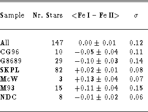
Table 6: Mean differences Fe I - Fe II in globular cluster giants
Data concerning the Fe ionization equilibrium are shown in Table 6 (click here)
which lists the mean differences between abundances derived from neutral and
singly ionized lines of Fe. These values have been computed both for the
total sample and for the different sub-samples studied. From this Table we
conclude that there is an excellent agreement between abundances derived from
Fe I and Fe II, with no trend with ![]() or [Fe/H]. The lack of any trend over
the whole range of temperature is very important, since in the past some
analysis (e.g., Pilachowski et al. 1983) claimed that a discrepancy was present
between these 2 iron abundances in stars cooler than 4300 K. The implication
was that in the very upper red giant branch the usual Local Thermodynamic
Equilibrium (LTE) assumption had to be released or, at least, carefully
verified by statistical equilibrium computations. Our results, however,
strongly confirm the recent study of Clementini et al.
(1995; see also the footnote below) that pointed out that
departures from LTE cannot significatively affect abundance analyses
for stars cooler than RR Lyrae variables.
or [Fe/H]. The lack of any trend over
the whole range of temperature is very important, since in the past some
analysis (e.g., Pilachowski et al. 1983) claimed that a discrepancy was present
between these 2 iron abundances in stars cooler than 4300 K. The implication
was that in the very upper red giant branch the usual Local Thermodynamic
Equilibrium (LTE) assumption had to be released or, at least, carefully
verified by statistical equilibrium computations. Our results, however,
strongly confirm the recent study of Clementini et al.
(1995; see also the footnote below) that pointed out that
departures from LTE cannot significatively affect abundance analyses
for stars cooler than RR Lyrae variables.
For the SKPL sample it should be noted again that in their
original papers both photometric gravities and ![]() values were
purposedly changed to obtain a match of the two [Fe/H] abundances within
0.05 dex.
values were
purposedly changed to obtain a match of the two [Fe/H] abundances within
0.05 dex.

Table 7: Dependence of the derived abundances on atmospheric parameters
Table 7 (click here) shows the dependance of the derived abundances from uncertainties in the adopted atmospheric parameters; this is obtained by re-iterating the analysis while varying each time only one of the parameters. To show how these sensitivities change with overall metal abundance, we repeated this exercise for both a metal-rich (star 8406 in 47 Tuc) and a metal-poor giant (star A61 in NGC 6752).
Entities of variations are quoted in Table 7 (click here): these
values are larger than errors likely present in the adopted atmospheric
parameters. This will be shown in the following discussion, where we will try
to provide reasonable evaluations
for the uncertainties in the adopted atmospheric
parameters. To this purpose, we compared expected scatters in Fe abundances
within individual clusters and differences between abundances provided
by neutral and singly ionized lines with observed values. Relevant data for
this last parameter can be easily obtained from
Table 6 (click here)![]() . For the reasons above mentioned, we omit from
the following discussion the value from the SKPL sample and we concentrate
instead on the other mean differences, for which the standard deviation
. For the reasons above mentioned, we omit from
the following discussion the value from the SKPL sample and we concentrate
instead on the other mean differences, for which the standard deviation ![]() represents the random errors contribution, and the error of
the mean (0.01
represents the random errors contribution, and the error of
the mean (0.01 ![]() 0.04) the contribution due to systematic errors.
0.04) the contribution due to systematic errors.
The relevance of systematic errors is always difficult to reliably assess. We do not think there are serious concerns related to the adopted gf scale. On the other side, uncertainties due to the adopted model atmospheres may be large since various important aspects (like convection, molecular opacities, and horizontal inhomogeneities) are far from being adequately known. Large trends of Fe abundances with excitation have been obtained in the analysis of field metal-poor giants by Dalle Ore (1992), Dalle Ore et al. (1996), Gratton & Sneden (1994), and Gratton et al. (1996), when using both BEGN and K92 model atmospheres. These trends suggest that currently available model atmospheres are not fully adequate for at least some metal-poor giants (see e.g. Castelli et al. 1996). While absolute abundances are quite sensitive to this source of errors, the comparison of relative abundances obtained with different model atmosphere grids (K92 and BEGN) suggests that our [Fe/H] values are not heavily affected. However, our analysis should obviously be repeated once improved model atmospheres for metal-poor giants become available.
We need to concern less about possible errors in the adopted temperature scale (in our
case, the CFP one). In fact, were the ![]() scale largely in error, we would
expect a rather large difference between average abundances provided by neutral
and singly ionized Fe lines. The values listed in Col. 2 of
Table 7 (click here) indicate that a systematic error of 100 K in the adopted
scale largely in error, we would
expect a rather large difference between average abundances provided by neutral
and singly ionized Fe lines. The values listed in Col. 2 of
Table 7 (click here) indicate that a systematic error of 100 K in the adopted
![]() 's would translate into a systematic difference of 0.2 dex between
abundances of Fe I and Fe II. Since the observed difference ranges from
0.02 dex to 0.13 dex (depending on the considered sample), we conclude that the
's would translate into a systematic difference of 0.2 dex between
abundances of Fe I and Fe II. Since the observed difference ranges from
0.02 dex to 0.13 dex (depending on the considered sample), we conclude that the
![]() scale cannot be systematically incorrect by more than 50 K.
scale cannot be systematically incorrect by more than 50 K.
Internal errors may be determined from a comparison with the observed scatter in our abundance determinations (of individual lines and of individual stars in each cluster). We will consider only errors in the EWs and in the adopted atmospheric parameters, while we regard internal errors in the adopted gfs as negligible.
The scatter of abundances from individual (Fe I) lines is 0.13, 0.11, 0.15,
0.15, 0.14 and 0.12 dex for the CG96, SKPL, G8689, McW92, M93 and NDC samples
respectively. These values for the
scatter can be ascribed to errors in the EWs of a few mÅ (see Sect. 3),
and yield mean
internal errors of 0.03 and 0.06 dex for Fe I and Fe II respectively. These
internal errors can be added quadratically and give a prediction
of about 0.07 dex for the scatter in the differences between abundances
derived from Fe I and Fe II lines. Since the observed scatter ranges
from ![]() to
to ![]() (depending on the adopted sample), additional
sources of errors are clearly present, probably related to the adopted values
for the atmospheric parameters (see Table 7 (click here) and discussion below).
(depending on the adopted sample), additional
sources of errors are clearly present, probably related to the adopted values
for the atmospheric parameters (see Table 7 (click here) and discussion below).
CFP V-K colours have errors of ![]() mag, which corresponds to
35-40 K using their calibration. This is the internal error of
mag, which corresponds to
35-40 K using their calibration. This is the internal error of ![]() 's for
stars within a cluster. When comparing stars in different clusters, the effects
of errors in the interstellar reddening should also be considered. Comparing
various estimates for the same cluster, we estimate an uncertainty of
's for
stars within a cluster. When comparing stars in different clusters, the effects
of errors in the interstellar reddening should also be considered. Comparing
various estimates for the same cluster, we estimate an uncertainty of
![]() mag in E(B-V), and 2.7 times larger in E(V-K). Hence,
there is an additional systematic error of
mag in E(B-V), and 2.7 times larger in E(V-K). Hence,
there is an additional systematic error of ![]() mag in the
mag in the ![]() \
colour (
\
colour (![]() K) systematic for all stars in a cluster (but random from
cluster to cluster) due to errors in the reddening. If we add these two
uncertainties quadratically, we estimate that the adopted
K) systematic for all stars in a cluster (but random from
cluster to cluster) due to errors in the reddening. If we add these two
uncertainties quadratically, we estimate that the adopted ![]() 's have internal
errors of
's have internal
errors of ![]() K. The same figures approximately hold for the B-V
colour, which is a less accurate temperature indicator (see e.g., Gratton
et al. 1996), but at the same time is measured with a precision better by a
factor of 5 than the V-K for bright globular cluster giants.
K. The same figures approximately hold for the B-V
colour, which is a less accurate temperature indicator (see e.g., Gratton
et al. 1996), but at the same time is measured with a precision better by a
factor of 5 than the V-K for bright globular cluster giants.
Table 7 (click here) suggests that most of the residual scatter in the
differences between Fe I and Fe II abundances may be attributed to random
errors in the adopted ![]() values.
values.
The adopted gravities were deduced from the location of the
stars in the CMD. Since
they were not deduced from the ionization equilibrium, one could think that
errors in ![]() and in
and in ![]() are not tied
are not tied![]() . But, as matter of fact, temperature
and gravity are not completely independent, since to derive
. But, as matter of fact, temperature
and gravity are not completely independent, since to derive ![]() from the
position of the star in the CMD we have to use the relationship
from the
position of the star in the CMD we have to use the relationship ![]()
![]()
![]() , i.e.:
, i.e.:
![]()
To estimate the order of magnitude of the errors affecting gravity, consider
the following:
In column 3 of Table 7 (click here) we investigate the effects of a variation
of 0.5 dex in the surface gravity; on the basis of the previous discussion, the
contribution from this column should be then divided by at least a factor of 3.
It is interesting to note that a larger error of ![]() would
explain the whole residual 0.11 dex in the random error. This is not the case,
though, since there is surely a contribution from errors in
would
explain the whole residual 0.11 dex in the random error. This is not the case,
though, since there is surely a contribution from errors in ![]() : this further
confirms that
: this further
confirms that ![]() is an overestimate, and the assumed value of
0.15 dex is reliable.
is an overestimate, and the assumed value of
0.15 dex is reliable.
For each star analyzed we have also random errors in the estimate of [A/H] due
to errors in ![]() , in gravity (of little entity) and in the measured EWs.
This kind of errors can be evaluated from independent analyses of the same
star. To this purpose, we can compare the results obtained for stars in
the same
cluster, since they are thought to share the same overall metallicity: the
rms deviation from the mean will give an idea of the uncertainties due to
random factors. The quadratic average is 0.06 dex and so they contribute very
little to the observed difference in the abundances from Fe I and Fe II (less
than 0.025 dex, from Table 7 (click here)).
, in gravity (of little entity) and in the measured EWs.
This kind of errors can be evaluated from independent analyses of the same
star. To this purpose, we can compare the results obtained for stars in
the same
cluster, since they are thought to share the same overall metallicity: the
rms deviation from the mean will give an idea of the uncertainties due to
random factors. The quadratic average is 0.06 dex and so they contribute very
little to the observed difference in the abundances from Fe I and Fe II (less
than 0.025 dex, from Table 7 (click here)).
The internal error in the ![]() is usually estimated from the comparison of
empirical and theoretical curve-of-growth; it is typically not larger than
0.2 km s
is usually estimated from the comparison of
empirical and theoretical curve-of-growth; it is typically not larger than
0.2 km s![]() for the giants analyzed, since the microturbulent velocity is
derived using Fe I lines both on the linear and saturation part of the
curve-of-growth. As above, an independent test of the random errors comes from
the comparison between the values obtained for the same star independently
analyzed. We obtained
for the giants analyzed, since the microturbulent velocity is
derived using Fe I lines both on the linear and saturation part of the
curve-of-growth. As above, an independent test of the random errors comes from
the comparison between the values obtained for the same star independently
analyzed. We obtained ![]()
![]() =0.17 km s
=0.17 km s![]() for the star C428 in
CG96 and in the G8689 sample; it confirms that the microturbulent velocity has
an error smaller than 0.2 km s
for the star C428 in
CG96 and in the G8689 sample; it confirms that the microturbulent velocity has
an error smaller than 0.2 km s![]() .
.
To conclude, we have to consider two kinds of errors: first, the internal,
random errors, that affect the comparison from star to star, and second, the
systematic errors, that give an idea of the reliability of our metallicity
scale, of the temperature scale adopted, etc. For the random errors, we have
seen that reasonable estimates are 50 K in ![]() , 0.15 dex in
, 0.15 dex in ![]() ,
0.06 dex in [A/H] and 0.2 km s
,
0.06 dex in [A/H] and 0.2 km s![]() in
in ![]() ; these errors will affect the
scatter of our data. As to systematic errors, we have only the indication
given by the difference in the abundances from neutral and singly ionized Fe
lines; from the previous discussion, we conclude that these errors are of the
same order of magnitude of random ones.
; these errors will affect the
scatter of our data. As to systematic errors, we have only the indication
given by the difference in the abundances from neutral and singly ionized Fe
lines; from the previous discussion, we conclude that these errors are of the
same order of magnitude of random ones.
Columns 6 and 7 of Table 7 (click here) list the uncertainties in the [Fe/H] ratios derived from the quadratic sum of the contributions from random and systematic errors, respectively. We remark that the changes in the parameters used to construct these columns are not those indicated in the Table, but the more realistic estimates obtained from the above discussion. From Table 7 (click here) we can estimate that the total uncertainty in our Fe I abundances (from which we derive the clusters metallicity) is about 0.11 dex for the most metal-poor stars, increasing to about 0.13 dex for the most metal-rich stars.