The reduced charge number ![]() is defined by
is defined by
![]()
where Z is the atomic number (i.e. nuclear charge in atomic units)
for which the range is ![]() .
. ![]() is usually
equal to the number of bound electrons N although on occasions it is
more convenient if
is usually
equal to the number of bound electrons N although on occasions it is
more convenient if ![]() as in the second example
(Fig. 2 (click here))
where
as in the second example
(Fig. 2 (click here))
where ![]() . Here we omit the neutral atom case and consequently
obtain a much better fit to the positive ion data points. The parameter C
is adjusted in order to optimise the spline fit. The plots we use are either
of type 2 (
. Here we omit the neutral atom case and consequently
obtain a much better fit to the positive ion data points. The parameter C
is adjusted in order to optimise the spline fit. The plots we use are either
of type 2 (![]() for large Z) or type 3
(
for large Z) or type 3
(![]() for large Z). The different types of plot are defined
and discussed by Burgess & Tully (1992).
for large Z). The different types of plot are defined
and discussed by Burgess & Tully (1992).
![]()
Figure 2: Fluorine sequence: ![]() ,
, ![]() , C = 1.8
, C = 1.8
Figure 1 (click here) concerns temperatures of maximum abundance
![]() for fluorine-like ions in conditions of coronal ionization
equilibrium. From Arnaud & Rothenflug's (1985)
tabulation we obtain
estimates of log(
for fluorine-like ions in conditions of coronal ionization
equilibrium. From Arnaud & Rothenflug's (1985)
tabulation we obtain
estimates of log(![]() ) for 10 ions in the sequence. Our spline fit
can be used to complete their tabulation for the intermediate
ions which they
did not consider. Here we input
) for 10 ions in the sequence. Our spline fit
can be used to complete their tabulation for the intermediate
ions which they
did not consider. Here we input ![]() and treat
it as a type 2 case. The optimised fit has C = 4.4 and rms error 0.38%.
Since we only wish to interpolate the data but not extrapolate them, we are
not concerned with the high Z limit point. In fact it does not exist
since there is a weak (logarithmic) divergence in this case.
and treat
it as a type 2 case. The optimised fit has C = 4.4 and rms error 0.38%.
Since we only wish to interpolate the data but not extrapolate them, we are
not concerned with the high Z limit point. In fact it does not exist
since there is a weak (logarithmic) divergence in this case.
Figure 2 (click here) deals with the ionization energy
I of fluorine-like ions. Since I increases like ![]() as Z tends to
as Z tends to
![]() , we treat this as type 2 by inputting
, we treat this as type 2 by inputting ![]() , with
I in
, with
I in ![]() . The limit point at
. The limit point at ![]() corresponding to
corresponding to
![]() is the hydrogenic value
is the hydrogenic value ![]() , while the
optimised fit (rms error 0.16%) is obtained with C = 1.8.
, while the
optimised fit (rms error 0.16%) is obtained with C = 1.8.
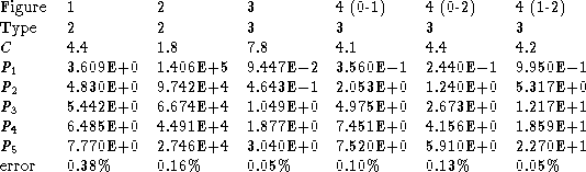
Table 1: Spline fitting parameters for the curves shown in the figures
![]()
Figure 3: Aluminium sequence: ![]() ,
, ![]() ,
C=7.8
,
C=7.8
Figure 3 (click here) shows our way of interpolating the ground term magnetic
dipole transition energies for the aluminium sequence. It is instructive to
compare this way of plotting the data with that used by
Edlén (1942) in his
Fig. 1 (click here). We invert the observed spin-orbit splitting
![]() of the
of the
![]() term, which Edlén (1942)
gives in
term, which Edlén (1942)
gives in ![]() in Table 2 (click here), and take the square root. This yields a quantity
in Table 2 (click here), and take the square root. This yields a quantity
![]() at high Z. The value of the
limit point for this type 3 plot is
at high Z. The value of the
limit point for this type 3 plot is
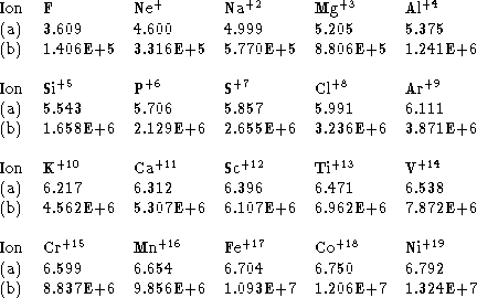
Table 2: (a) Log(![]() from the spline fit shown in Fig. 1.
from the spline fit shown in Fig. 1.
![]() is the temperature of maximum coronal abundance
for F-like ions.
(b) Ionization energy in
is the temperature of maximum coronal abundance
for F-like ions.
(b) Ionization energy in ![]() for F-like ions deduced
from the spline
fit shown in Fig. 2. The results given here are calculated using data from
Table 1
for F-like ions deduced
from the spline
fit shown in Fig. 2. The results given here are calculated using data from
Table 1
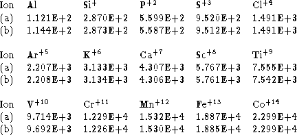
Table 3: Transition energy in ![]() for the fine structure splitting
in the ground configuration of aluminium and Al-like ions. (a) Using the
spline interpolation data given in Table 1. (b) Using Edlén's (1964)
extrapolation formula
for the fine structure splitting
in the ground configuration of aluminium and Al-like ions. (a) Using the
spline interpolation data given in Table 1. (b) Using Edlén's (1964)
extrapolation formula
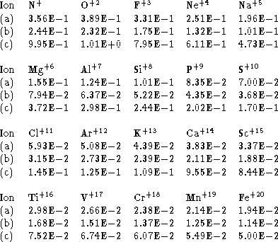
Table 4: Fine structure collision strengths ![]() at zero
energy for the ground
at zero
energy for the ground ![]() term in C-like ions.
(a)
term in C-like ions.
(a) ![]() ;
(b)
;
(b) ![]() ;
(c)
;
(c) ![]() .
Results obtained using the interpolating spline fit given in Table 1
.
Results obtained using the interpolating spline fit given in Table 1
![]()
and is deduced from the well-known
expression for the spin-orbit splitting given by Edlén (1964,
p. 167), viz.
![]()
4
where the screening parameter s' > 0 is a finite quantity which
varies slowly with Z. The optimised spline fit (rms error of 0.05%) is
obtained when C = 7.8. Edlén's (1964)
extrapolation formula for Z-s' as a
function of Z is given by the pair of equations
![]()
![]()
which reduces to finding the roots of the cubic
equation (Maple 1995)
![]()
where
![]()
and
![]()
Only one of the roots of (5) is a physical solution, and its
range of validity as a function of Z is limited, since for ![]() the
screening parameter s' becomes negative.
the
screening parameter s' becomes negative.
Figure 4 (click here) shows the compacting and interpolation of
Blaha's (1969) distorted
wave results for three fine structure collision strengths at
threshold energy
in the carbon sequence. The transitions are between the lowest three levels.
Blaha gives results for neutral carbon and 7 ions
in the sequence.
Here we take ![]() and input
and input ![]() which
decreases like
which
decreases like ![]() as
as ![]() . The high Z limits for
. The high Z limits for
![]() are from Saraph et al. (1969).
are from Saraph et al. (1969).
The five knot values ![]() and C parameter
for each of the spline curves shown in Figs. 1 to 4
are given in Table 1 (click here).
By means of the program FUNCTION SPLINE
and C parameter
for each of the spline curves shown in Figs. 1 to 4
are given in Table 1 (click here).
By means of the program FUNCTION SPLINE ![]() ,
(see Burgess & Tully's 1992 Appendix), it is
possible to interpolate the
reduced data points shown in the figures. Notice that
,
(see Burgess & Tully's 1992 Appendix), it is
possible to interpolate the
reduced data points shown in the figures. Notice that ![]() and by using the definition of
and by using the definition of ![]() in terms of
in terms of ![]() and
C, and knowing the type of plot one can obtain A(Z).
and
C, and knowing the type of plot one can obtain A(Z).
The interpolated results given in Tables 2 (click here), 3 (click here) and 4 (click here) are calculated using data in Table 1 (click here) and the spline program from Burgess & Tully (1992).
![]()
Figure 4: Carbon sequence: ![]() ,
, ![]() ,
,
![]() ,
, ![]() ,
, ![]()