3 Linear regularization methods and the global PSF

A classical approach to the solution of linear ill-posed problems is the so-called regularization theory. In its general form it consists in the minimization of a functional which is obtained from the discrepancy functional by adding a penalty term. This is, in general, the square of the norm of a differential (finite difference) operator acting on the image to be restored. In the case of deconvolution problems no one of the various form of regularization provides an extrapolation of the Fourier transform outside the band of the image and all provide in practice very similar result. Therefore we give here the most simple one which consists in taking as penalty term the energy of the object and which is usually known as Tikhonov Regularization (TR) (Engl et al. 1996). In such a case the functional to be minimized is the following one

$$\Phi_\mu(\vec{f})= \sum_{j=1}^p \Vert\vec{A}_j\vec{f}-\vec{g}_{s,j}\Vert^2 + \mu \Vert\vec{f}\Vert^2$$ (11)

where $\mu$ is a positive number called regularization parameter. When $\mu$ tends to zero this functional tends to the discrepancy functional.

For any given value of $\mu$ there exists a unique image $\vec{f}^{(\mu)}$which minimizes the functional and is the unique solution of the normal equation

$$\left( \sum_{j=1}^p\vec{A}_j^{\rm T} \vec{A}_j + \mu \vec{I} ... ... \vec{f}^{(\mu)}= \sum_{j=1}^p\vec{A}_j^{\rm T} \vec{g}_{s,j},$$ (12)

which can also be easily solved by means of the DFT. The result is

$$\hat f^{(\mu)}(m,n)=\sum_{j=1}^p {{\hat K_j^\ast(m,n)}\over{\mid \hat K(m,n) \mid^2 + \mu}} \hat g_{s,j}(m,n)$$ (13)

with $\vert\hat K(m,n)\vert^2$ defined in Eq. (9).

This equation defines the family of the regularized solutions. As concerns their dependence on the regularization parameter, we recall that there exists an optimum value of $\mu$, in the sense that it minimizes the restoration error. Several methods have been proposed for its estimation (see I). However, in the practice of LBT imaging, the problem of the choice of the optimal value of $\mu$ can be satisfactorily solved in the following way. As follows from Eq. (13), if the DFTs of the images and of the PSFs have been computed and stored, then, for each value of $\mu$, the computation of $\vec{f}^{(\mu)}$ requires essentially the computation of one inverse FFT. Therefore the method can be used routinely for a fast inversion of the data and the choice of the best value of $\mu$ can be performed interactively by the user.

It is possible to estimate the resolution achievable with a given set of observations without performing explicit data inversion. Such a result can be obtained by generalizing to the LBT problem the concept of global PSF introduced in I. The global PSF is the PSF of two linear systems in cascade: the first is the imaging system (the LBT in our case) while the second is the linear filter corresponding to the TR restoration method.

If we insert the images $\hat{g}_{s,j}(m,n)$, as given by Eqs. (6) and (3), into Eq. (13), we obtain

 

$$\hat f^{(\mu)}(m,n) {{\mid \hat K(m,n)\mid^2}\over { \mid \hat K(m,n)\mid^2 +\mu}}\hat f_0(m,n)$$ =

$$\sum_{j=1}^p {{ \hat K_j^\ast(m,n)}\over{\mid \hat K(m,n)\mid^2+\mu}}\hat w_j(m,n).$$ + (14)

This equation has a structure similar to that of Eq. (3) after background subtraction. Indeed, the DFT of the restored image $\vec{f}^{(\mu)}$ consists of two terms: the first is the DFT of the object multiplied by the transfer function

$$\hat K^{(\mu)}(m,n)={{\mid \hat K(m,n)\mid^2}\over { \mid \hat K(m,n)\mid^2 +\mu}} ;$$ (15)

the second is a contribution due to the noise. Therefore it is quite natural to define $\hat K^{(\mu)}(m,n)$ as the global transfer function and, accordingly, to define its inverse DFT, $\vec {K}^{(\mu)}$, as the global PSF.

Figure 1: Gray level representation of the global transfer function of Eq. (15) for various sets of baseline orientations: a) three directions spaced by 60$^\circ$; b) six directions spaced by 30$^\circ$; c) three directions spaced by 45$^\circ$; d) six directions spaced by 18$^\circ$. In the cases a) and c), $\mu=3~10^{-3}$ while, in the cases b) and d), $\mu=6~10^{-3}$

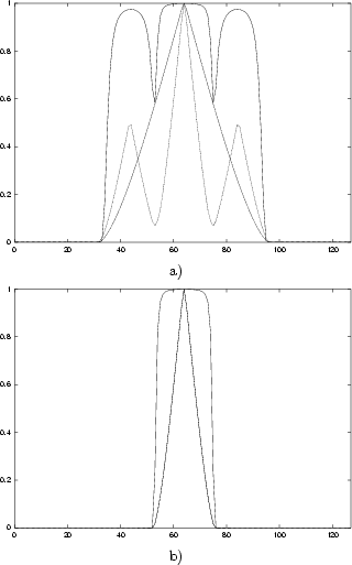Figure 2: a) Horizontal cut (full line) of the global transfer function of Fig. 1d or Fig. 1b, compared with a cut of the transfer function of a 22.8 m telescope (dashed line) and the cut, along the baseline, of the transfer function of the LBT interferometer (dotted line). b) Vertical cut (full line) of the global transfer function of Fig. 1d, compared with the cut, along the direction orthogonal to the baseline, of the transfer function of the LBT interferometer (dash-dotted line). The latter coincides with the cut of the transfer function of a 8.4 m telescope

It is evident that the global transfer function has a support coinciding with the coverage of the u-v plane provided by the observations we use and that, over this support, modulates the Fourier transform of the object in a way depending on the value of $\mu$. We recall that the optimal value of this parameter depends on the amount of noise: smaller noise corresponds to smaller values of $\mu$, hence to more detailed restorations.

In order to quantify the previous remarks we consider a few possible situations, by assuming diffraction limited PSFs of the LBT interferometer, i.e. cosine-modulated Airy functions. They are normalized in such a way that their zero frequency component is 1. In addition their FWHM is about 4 pixels in the direction of the baseline and about 11.2 pixels in the orthogonal direction (with the same units the FWHM of a 22.8 m pupil is 5.5 pixels). The interferometric PSFs are computed for p equispaced orientations: in one case they cover 180$^\circ$ while in the other they cover 90$^\circ$. In both cases we consider p = 3 and p = 6. As concerns the value of the regularization parameter, from a criterion proposed in Miller (1970) it follows that it is roughly proportional to p. We take $\mu = p~10^{-3}$, a value which roughly corresponds to the optimal value used for the first numerical example of Sect. 6.

In Fig. 1 we give pictures of the global transfer functions corresponding to the situations indicated above. In these figures the circular bands of the 8.4 m and of the 22.8 m mirror are evident. The lower panels of Fig. 1 show a striking similarity with the situation encountered in limited angle tomography which, as it is well known, does not allow satisfactory image restorations. However the results of Sect. 6 indicate that the situation is more favourable in the case of LBT, mainly as a consequence of the information carried out by the 8.4 m mirror.

In Fig. 2 we plot horizontal and vertical cuts of the global transfer function of Fig. 1d, both through the centre of the inner disc. The horizontal cut, represented in Fig. 2a (full line), is compared with a cut of the transfer function of a 22.8 m telescope (dashed line) and with the cut, along the direction of the baseline, of the transfer function of the LBT interferometer (dotted line). Thanks to the use of a restoration method for producing the final image, the global transfer function of LBT assures a more accurate transmission of the Fourier components of the object than the transfer function of a 22.8 m telescope. As a consequence, in the case of a complete coverage as in Fig. 2b, the FWHM of the global PSF is about 2.8 pixels, against the 5.5 pixels of the PSF of a 22.8 m telescope. The price to be payed is that the central peak of the global PSF is surrounded by rather important negative rings. We observe that similar results could be obtained by applying TR to the images of a hypothetical 22.8 m telescope.

In Fig. 2b the vertical cut of the global transfer function of Fig. 1d (full line) is compared with the cut of the transfer function of the LBT interferometer along the direction orthogonal to the baseline (dash-dotted line). The latter coincides with a cut of the transfer function of a 8.4 m telescope. Again the use of restoration methods implies a more accurate transmission of the Fourier components of the object. In addition, if we compute the global PSF corresponding to the transfer function of Fig. 1d, we find that its FWHM in the vertical direction is about 4 pixels which is much smaller than that of a 8.4 m telescope (11 pixels). This effect may be due to the contributions coming from other directions in the u-v plane and is in agreement with the result of a simulation reported in Sect. 6 (see Fig. 3d).