6 Numerical results

We have implemented the five restoration methods discussed in the previous sections: TR, as the prototype of the linear methods used for regularizing least-squares solutions; PL and ISRA, as regularization methods for constrained least-squares solutions with the positivity constraint; LR/EM and its accelerated version OS-EM. The methods TR, PL and ISRA apply, in principle, to the case of white Gaussian noise but are commonly used also for the restoration of images corrupted by Poisson and Gaussian noise.

All the algorithms include one or more parameters whose values must be optimized by means of numerical simulations, according to the tasks established by the users. This procedure may be called the training of the algorithm and the tasks may be defined through the so-called Figures of Merit (FOM).

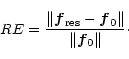
In this paper, we use three different FOMs. The first reflects the ability of the algorithms to minimize the restoration error (RE), i.e. the relative RMS discrepancy between the true object $\vec{f}_0$ and its restored version $\vec{f}_{{\rm res}}$

$$RE={{\Vert\vec{f}_{\rm res}-\vec{f}_0\Vert}\over{\Vert\vec{f}_0\Vert}}\cdot$$ (24)

In addition we introduce two different photometric FOMs to evaluate the photometric efficiency of the various methods. The first is related to the flux on a set of Regions Of Interest (ROI) while the second evaluates the photometric accuracy in the case of a single star or of a cluster of stars.

If the ROIs are R₁, R₂,..., R_r, then in each one the fluxes of the original image and of the restored one are given by:

$$\Phi_l=\sum_{m,n\in R_l} f_0(m,n); \ \ \Phi_l^{({\rm res})}=\sum_{m,n\in R_l} f_{{\rm res}}(m,n)$$ (25)

with l = 1, 2,...,r, so that we can define the Flux Error (FE) as follows:

$$FE={1\over r} \sum_{l=1}^r{ {\mid \Phi_l - \Phi_l^{({\rm res})}\mid}\over{\Phi_l}}\cdot$$ (26)

As concerns the second photometric FOM, let us assume that we are considering a set of s stars corresponding to the regions S₁, S₂,..., S_s. Then, for each star, we can compute the magnitude as follows:

$$m_l= -2.5~{\rm log}_{10}\left(\sum_{m,n\in S_l} {{f_0(m,n)} \over {f_b}}\right)$$ (27)

( l = 1, 2,...,s), where f_b is the sky flux per (arcsec)². If we compute the magnitude of the reconstructed star $m_l^{({\rm res})}$ in a similar way, we define the Average Magnitude Error (AME) as follows

$$AME = {1\over s} \sum_{l=1}^s \mid m_s-m_s^{({\rm res})}\mid .$$ (28)

In our numerical simulations we use the same objects and images of previous papers (Correia & Richichi 1999; Bertero & Boccacci 2000). Therefore perfect AO correction is assumed and the interferometric PSFs are cosine-modulated Airy functions (whose FWHM in the direction of the baseline is about 4 pixels). The simulated observations, performed in R band, are obtained by convolving the diffraction-limited PSFs with the object and by adding suitable background and noise (Poisson plus read-out) to the result. Details on the values of the relevant parameters (integration times, sky brightness etc.) can be found in Correia & Richichi (1999).

The first object is an image $128\times 128$ of the spiral galaxy NGC 1288, which is shown in Fig. 3a, where the white squares indicate the ROIs used for the computation of FE. For this object we have computed three sets of simulated images corresponding to 4, 6 and 8equispaced values of the parallactic angle between $0^\circ$ and $180^\circ$. Since the magnitude of the galaxy is set to m_r = 19, this leads to approximately 2 10⁷ photons per long exposure images and a peak SNR of 80.

 

 

Table 1: Summary of the results obtained for the galaxyNGC 1288 by means of the methods implemented in this work. For each method we report the minimum value of RE and FE and the corresponding value of the regularization parameter $\mu _{{\rm opt}}$ or of the number of iterations $k_{{\rm opt}}$

method	p	$k_{{\rm opt}}$	RE	$k_{{\rm opt}}$	FE
		or $\mu _{{\rm opt}}$		or $\mu _{{\rm opt}}$
	4	$6.5\ 10^{-3}$	0.049	$8.0\ 10^{-4}$	0.0160
TR	6	$7.3\ 10^{-3}$	0.049	$3.5\ 10^{-3}$	0.0120
	8	$8.8\ 10^{-3}$	0.043	$3.7\ 10^{-3}$	0.0040
	4	278	0.048	273	0.0137
PL	6	329	0.044	361	0.0139
	8	392	0.042	467	0.0024
	4	373	0.046	408	0.0157
ISRA	6	487	0.042	569	0.0126
	8	519	0.040	670	0.0030
	4	314	0.044	295	0.0138
LR/EM	6	380	0.040	381	0.0126
	8	393	0.039	411	0.0059
	4	79	0.044	76	0.0140
OS-EM	6	64	0.040	62	0.0131
	8	50	0.039	52	0.0050

For this example we have investigated the behaviour of two FOMs, RE and FE. As functions of the regularization parameter (TR) or of the number of iterations (PL, ISRA, LR/EM, OS-EM) both exhibit a minimum (hence an optimal restoration from the point of view of that FOM). The minima of RE and FE do not occur for the same value of the parameters. The results are summarized in Table 1.

A few comments on these results are appropriate. First, the restoration error is rather small (as a consequence of the good SNR of the simulated images as well as of the good coverage of the u-v plane) and is approximately the same for all methods. Second, the restoration error decreases for increasing number of images, as it is expected, even if the improvement is not very spectacular (a gain of $0.5 \%$ from 4 to 8images). We also notice that the optimal value of the regularization parameter, as well as the optimal value of the number of iterations, increases for increasing number of images (except for OS-EM). An argument justifying this behaviour is given in Sect. 3. In the case of OS-EM, as already shown in Bertero & Boccacci (2000) the number of iterations decreases when the number of images increases, in such a way that the computation time does not significantly depends on the number of images.

Similar remarks apply also to the case of FE, which measures the local accuracy of the restoration. FE is always smaller than RE and, in general, this result is obtained with a smaller value of the regularization parameter or a higher number of iterations. In addition we observe a strong reduction of FE when using eight images instead of four or six.

As already remarked all methods provide in practice the same restoration error. This result is due to the fact that we are restoring a diffuse object with a rather large (and varying) background, so that the positivity constraint is not active (see I for a discussion). In similar cases one can choose the restoration method on the basis of the computational cost.

 

 

Table 2: Restoration errors corresponding to different values of the total parallactic angle. The results are obtained for the galaxy NGC 1288, using four equispaced images for each value of the total angle

Total	(TR)		(PL)		(LR/EM)
angle	$\mu _{{\rm opt}}$	RE	$k_{{\rm opt}}$	RE	$k_{{\rm opt}}$	RE
$135 ^\circ$	$4 \ 10^{-3}$	0.049	278	0.044	314	0.044
$93 ^\circ$	$7 \ 10^{-3}$	0.053	256	0.052	288	0.048
$63 ^\circ$	$7 \ 10^{-3}$	0.056	253	0.056	309	0.051

We have used our codes also for testing, on the particular example of the galaxy NGC 1288, the effect of incomplete coverage of the u-v plane. We have assumed four equispaced images within total parallactic angles (difference between the angles of the two extreme orientations of the baseline) of $135 ^\circ$, $93 ^\circ$ and $63 ^\circ$ (the first case corresponds to the first case of Table 1). In Table 2 we report, for simplicity, only the results obtained with TR, PL and LR/EM. The notations are those used in Table 1. Again all methods provide essentially the same restoration error and it is rather surprising to find that this error does not increase dramatically when the total parallactic angle decreases. We remark that the case of $93 ^\circ$ corresponds approximately to the coverage of the u-v plane shown in Fig. 1d (after a rotation of about $45^\circ$).

A visual confirmation of the result is provided by Fig. 3 where two examples of restorations obtained by means of LR/EM are shown. Figure 3c is obtained using 8 equispaced images covering a total parallactic angle = $180^\circ$ while Fig. 3d is obtained with 4 equispaced images covering a total parallactic angle = $63 ^\circ$. These pictures suggest that an incomplete coverage of the u-v plane may not influence dramatically the general quality of the restored image, even if details recovered in the case of complete coverage are not recovered in the other one.

Figure 3: a) Original image of the galaxy NGC 1288. The white squares indicate the ROIs used to evaluate the FOM defined in Eq. (54). b) One of the simulated LBT images (parallactic angle = 0$^\circ$). c) Best restoration provided by the LR/EM method, using 8 equispaced images covering an angle = 180$^\circ$. d) Best restoration provided by the LR/EM method, using 4 images covering an angle = 63$^\circ$

The second example we consider is a simulation of binary stars of different relative magnitude. In the synthetic object each star is located in one pixel, with a separation of about 14 pixels which is about 3.5 times the diffraction limit in the direction of the baseline. Moreover two cases are investigated: 1) the magnitudes of the two stars are 27.5 and 30 and the average peak SNR in the images is 11.3 for the main star and 3.5 for the companion; 2) the magnitudes are 29 and 30 while the corresponding average peak SNRs are 5.5 and 3.5 respectively. Also for these examples we have computed sets consisting of 4,6 and 8 equispaced observations. Moreover, for TR, PL and ISRA the constant background has been subtracted from the simulated LBT images to obtain the subtracted images defined in Eq. (6). In the case of ISRA the negative values of $\vec{A}^{\rm T}_j\vec{g}_{s,j}$ have been set to zero. As concerns LR/EM and OS-EM, background subtraction is not needed because the value of the background is inserted directly in the algorithm, as indicated in Sect. 5. However, since the background is not very large, the computed images $\vec{g}_j$ can take small negative values in a few pixels as a consequence of the white Gaussian noise simulating the read-out noise. These values are set to zero in order to avoid instabilities of the algorithm.

 

 

Table 3: Summary of the results obtained for the binary star 27.5-30 by means of the methods implemented in this work. The * indicates that the quoted number of iterations does not correspond to the minimum of the FOM (see the text)

method	p	$k_{{\rm opt}}$	RE	$k_{{\rm opt}}$	AME
		or $\mu _{{\rm opt}}$		or $\mu _{{\rm opt}}$
	4	$1.0\ 10^{-3}$	0.922	$1.2\ 10^{-2}$	0.0294
TR	6	$1.0\ 10^{-3}$	0.913	$1.6\ 10^{-2}$	0.0375
	8	$1.0\ 10^{-3}$	0.911	$2.5\ 10^{-2}$	0.0345
	4	1000*	0.753	1000*	0.1080
PL	6	1000*	0.747	223	0.0579
	8	1000*	0.753	234	0.0362
	4	1000*	0.759	516	0.0501
ISRA	6	1000*	0.897	520	0.0109
	8	1000*	0.674	931	0.0072
	4	1000*	0.063	254	0.0448
LR/EM	6	1000*	0.047	223	0.0064
	8	1000*	0.032	158	0.0008
	4	1000*	0.043	64	0.0439
OS-EM	6	1000*	0.035	32	0.0099
	8	376	0.024	16	0.0029

 

 

Table 4: Summary of the results obtained for the binary star 29-30 by means of the methods implemented in this work. The * indicates that the quoted number of iterations does not correspond to the minimum of the FOM (see the text)

method	p	$k_{{\rm opt}}$	RE	$k_{{\rm opt}}$	AME
		or $\mu _{{\rm opt}}$		or $\mu _{{\rm opt}}$
	4	$1.4\ 10^{-2}$	0.956	$1.8\ 10^{-2}$	0.0198
TR	6	$1.2\ 10^{-2}$	0.934	$2.8\ 10^{-2}$	0.0054
	8	$1.3\ 10^{-2}$	0.936	$2.6\ 10^{-2}$	0.0128
	4	1000*	0.769	199	0.0412
PL	6	1000*	0.756	162	0.0441
	8	1000*	0.765	221	0.0166
	4	1000*	0.394	135	0.0429
ISRA	6	1000*	0.231	82	0.0380
	8	1000*	0.334	97	0.0694
	4	1000*	0.191	268	0.0310
LR/EM	6	1000*	0.193	266	0.0323
	8	1000*	0.152	186	0.0350
	4	1000*	0.148	69	0.0187
OS-EM	6	1000*	0.142	44	0.0300
	8	1000*	0.128	23	0.0454

The five implemented methods have been applied to the three sets of observations for each one of the two cases. The FOMs considered are RE and AME. The results are reported in Table 3 for the first case and in Table 4 for the second one. From the point of view of RE, the number of iterations needed for reaching the minimum is much larger than in the case of the galaxy NGC 1288. This is a general feature of iterative methods: point-like objects need much more iterations than diffuse objects. In addition the minima are usually very flat and, for this reason, in many cases we stopped the procedure after 1000 iterations. The results we have obtained may be summarized by saying that only in the case of LR/EM and OS-EM the restoration error RE decreases when the number of images increases. These two methods also provide a much smaller value of RE than the three others. Moreover RE is smaller in the case of example 1) (that with the higher SNR) than in the case of example 2), as it is expected.

As concerns AME, defined in Eq. (28), it has been computed on squares of $5 \times 5$ pixels, centred on the pixels of the two stars. The results are shown again in Table 3 and Table 4 for the two cases. It is not always true that the value of AME decreases with increasing number of iterations, even if it is true for LR/EM and OS-EM in the case of the binary with the higher SNR. In the case of low SNR, quite surprisingly TR is the method providing the best results. In general we observe fluctuations across the various methods but a very promising result is that, for reaching the minimum of AME, we need a quite small number of iterations, especially in the case of OS-EM.

The fluctuations indicated above may be due to the fact that, even if AME is small (the reported values correspond to an error on the fourth significant digit), it may be strongly influenced by noise. Therefore, in order to check this point, we have evaluated the noise dependence of AME by restoring images obtained with five different noise realizations (including that corresponding to the results reported in Table 4) and by computing the minimum value of AMEfor all these cases.

We restrict the analysis to the binary of Table 4, assuming six observations and using only ISRA, LR/EM and OS-EM. It turns out that the value of AME is always small (in general smaller than the value reported in Table 4) but strongly affected by the change in noise realization. For each method we have computed the average value and standard deviation of AME and the results are the following : ISRA, $0.022 \pm 0.012$; LR/EM, $0.017 \pm 0.012$; OS-EM, $0.015 \pm 0.011$. The three methods provide essentially the same results and, in all cases, the standard deviation of AME is approximately equal to its average value.