4 Analysis of ground contamination

In the long-wavelength regime of the GEM experiment, there are two main sources of contamination, aside from Galactic stray radiation, which affect invariably the antenna noise temperature of the sky. These are the emissions of the ground and the atmosphere. The latter, being a factor of at least 20þdB smaller than the former, can be safely considered to be an elevation-dependent contribution to the signal level of the main beam. The ground contamination, on the other hand, requires a precise knowledge of the spillover and diffraction sidelobes of the feed in order to discriminate its contribution to the overall antenna noise temperature. In this section, we apply the geometric diffraction model developed in Paper I in order to account for the effect of shielding in the estimates of the ground signal. The shields are (see Fig. 1) a 5-m high fence, inclined at $50\ifmmode^\circ\else\hbox{$^\circ$ }\fi$ from the ground and standing at 6.4 m from the pivot point of the dish, and a halo of aluminum panels extending 2.1 m from the dish petals. The fence attenuation was estimated at the 10-dB level for 408MHz radiation, but below 1 dB at 1465MHz.

4.1 Model predictions

Our analytical tools enable us to estimate, as a function of the zenith angle Z, the amount of ground contamination due to the unshielded and diffracted components. The estimates, in units of antenna temperature, are given according to Fresnel and Fraunhofer diffraction theories in order to test for near and far-field effects in the range $0\ifmmode^\circ\else\hbox{$^\circ$ }\fi\le Z\le 45\ifmmode^\circ\else\hbox{$^\circ$ }\fi$. The asymmetry of the feed patterns introduces an additional complication, since the solid angle over which the ground temperature is distributed (assumed to be the field of view below the upper edge of the fence) is seen through a sidelobe structure that depends on the orientation of the $\phi$-plane of the feed. Therefore, a family of 24 profiles was prepared for each feed by rotating the $\phi$-plane in $15\ifmmode^\circ\else\hbox{$^\circ$ }\fi$ steps around the beam axis. For a tilted dish, the $\phi=0\ifmmode^\circ\else\hbox{$^\circ$ }\fi$ reference directions of Fig. 7 correspond to the line of sight which clears off the edge of the halo at the smallest Z angle. Figures 10 and 11 display the model estimates assuming a 10 dB attenuation from the fence (as in the 408 MHz case) in the presence and absence of the halo, respectively. Figures 12 and 13 describe the situation of the 1465MHz channel, for which the model fence provides no significant attenuation. The upper and lower envelopes of each family of profiles have been identified along with some other profiles. The orientations of the 408MHz and 1465MHz feed patterns that produce these upper and lower envelopes are indicated with labelled arrows in Fig. 7.

Figure: Predicted antenna noise temperature due to transmitted and diffracted ground radiation in a one-shielded (fence) GEM experiment at 408MHz. The diffracted components were calculated in both the Fresnel (thin lines) and the Fraunhofer (thick lines) regimes. The beam pattern asymmetry of the backfire helices gives rise to families of profiles, some of which have been labelled according to the $\phi$-plane orientation of the feed. All the profiles fall into 4 sets, each of which has been drawn according to the sequence of line types indicated by $P_{\rm n}(\theta ,\phi )$

Figure: Predicted antenna noise temperature due to transmitted and diffracted ground radiation in the double-shielded GEM experiment at 408MHz. Two additional triple-sets of profiles have been included to show the Fresnel and Fraunhofer estimates at 1465MHz for $\phi=12\ifmmode^\circ\else\hbox{$^\circ$ }\fi$ using a 7.91(+0.35-0.32)-dB attenuating fence and raised 80þcm above the ground as discussed in Sect. 5.2. Legend and label explanations are as in Fig. 10

Figure: Predicted antenna noise temperature due to transmitted and diffracted ground radiation in a one-shielded (no halo) GEM experiment at 1465MHz. Legend and label explanations are as in Fig. 10. Since the assumed attenuation of the fence is small, 0.3þdB, the plotted profiles represent an effectively unshielded case

Figure 13: Predicted antenna noise temperature due to transmitted and diffracted ground radiation in the double-shielded GEM experiment (an effectively one-shielded, fenceless, configuration) at 1465MHz. Legend and label explanations are as in Fig. 10

  
4.2 Ground contamination scenarios

Figures 10 through 13 characterize four types of ground contamination scenarios: (1) fence-shielded in Fig. 10, (2) double-shielded in Fig. 11, (3) unshielded in Fig. 12 and (4) halo-shielded in Fig. 13. The distinction is clear enough to show how the amount of shielding and the wavelength-dependent strength of the diffraction effects shape the ground contamination profiles. Thus, as we proceed from a weakly-diffracting and unshielded antenna scenario to a strongly-diffracting and double-shielded one, far-field diffraction effects give way to near-field ones. In doing so, the distance-dependent calculations with the Fresnel approach become more difficult to be matched by the Fraunhofer approximations, whose typical overestimating power is further increased.

Shielded scenarios produce also profiles with a tendency to resemble the underlying variation of the solid angle that exposes the ground for a given Z (see Fig. 6 in Paper I). In particular, when Z is large enough to expose unscreened ground below the fence, the corresponding profile shows a marked increase in ground signal. It should be noted that the profiles obtained with the Fraunhofer formalism in the double-shielded scenario of Fig. 10 deviate from these generalized description, since one expects the role of near-field diffraction at the longer wavelength and at the innermost shield to become significant.

The composition of the ground contamination profiles in terms of their transmitted and diffracted components can also be investigated by analyzing the symmetrized responses $P_{\rm n}(\theta)$. The diffraction model that we are using does not produce, however, separate estimates of transmitted and diffracted components in the Fresnel regime. Unlike in the Fraunhofer regime, where both components are obtained independently, the Fresnel convolution integral for calculating the contamination by the halo (or of the dish in the unshielded scenario) produces a transmission-embedded result. Nevertheless, in order to obtain an equivalent form of diffraction component, we have subtracted from the convolved result the same transmitted component as in the Fraunhofer regime. In a very realistic sense, the definition of a spillover sidelobe reduces to the sidelobe level that is not modified by the presence of a physical obstruction along the line of sight of the feed and within the angular range of the ground temperature distribution. This analytical construct allows us to plot in Fig. 14 the ratio $R_{\rm t}$ of the transmitted component to the total ground contamination in the Fresnel regime.

The reason why the unshielded scenario in Fig. 14 produces anomalous $R_{\rm t}>1$ values is a consequence of the above given definition for the spillover component. This definition implies that the diffraction sidelobes (whose sidelobe level is modified) can actually suppress, rather than enhance, the spillover ones. From the point of view of a Fresnel diffraction pattern, this behavior is readily understood as the restriction imposed by the ground temperature distribution on the angular range spanning the relative power response of the feed. The restriction sets effectively an upper cut-off in the amplitudes of the crests that characterize the rippling profile of this response (see, for example, Fig. 4 in Paper I). Thus, if the cut-off is sufficiently low the overall relative power response can fall below unity. This spillover suppression is also present in the other scenarios, but is not dominant and, as expected from the geometrical argument above, it originates in the portion of the halo or dish hidden from the outside by the structure of the fence. The effect is stronger in the absence of the shields and it becomes more pronounced at the shorter wavelength. Similar calculations with a relatively lower sidelobe structure also demonstrated that in order for spillover suppression to set in, the level of the relevant sidelobes cannot be made arbitrarily small.

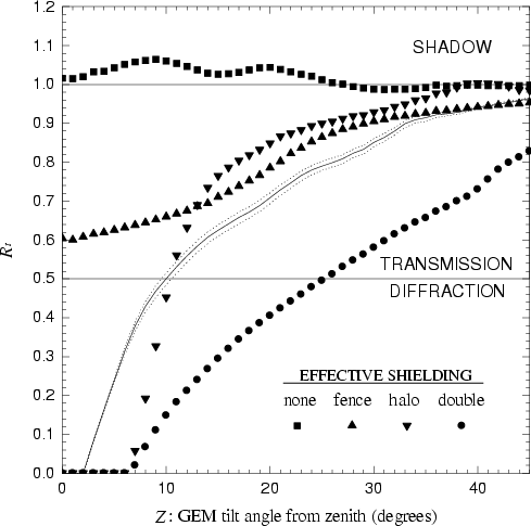Figure: The four ground contamination scenarios in terms of the ratio $R_{\rm t}$ of the transmitted component to the total ground contamination in the Fresnel regime. In the shadow region, spillover suppression by the diffraction sidelobes nearest to the ground dominate the diffracted component. The line and dotted curves mark the double-shielded case at 1465MHz discussed in Sect. 5.3

Although transmission dominates the ground contamination at large Z, the $R_{\rm t}$ curves in Fig. 14 indicate that diffraction becomes the dominant component at lower Z as the amount of shielding is also increased. We can quantify the relevance of the spillover sidelobes by introducing a transmission factor $Q_{\rm n}$ (the normalized integral under the $R_{\rm t}$ curves). Accordingly, a thoroughly spillover-dominated scenario would result in $Q_{\rm n}=1$, whereas a fully diffraction-dominated case would yield $Q_{\rm n}=0$. Table 2 lists the transmission factor in the four shielding scenarios analyzed in this section. Only the double-shielded scenario may be recognized to be dominated by the diffraction sidelobes.

Finally, it should be stressed that the estimates given in this section have assumed from the start that the ground temperature distribution is an isotropic field of radiation regardless of the horizon profile. As we saw in Sect. 2 this assumption is a valid one for a contaminating signal free of horizon-dependent variations, i.e. for a truly effective double-shielded scenario. Although possible, but not desirable for experimental reasons (horizontally striped maps), the convolution of the beam pattern with an anisotropic ground temperature distribution would yield a more realistic estimate in the other three scenarios. In these cases, a set of profiles like the ones shown in Figs. 10, 12 and 13 would have to be assembled for each particular azimuth.