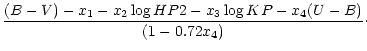
Equation (1) can be used to determine E(B-V) once all the observed indices are known. Since it is a first order equation both in (B-V) and (U-B) we may solve analytically for E(B-V), rather than by iteration, as it is necessary with the Schuster & Nissen calibration. By adopting the reddening slope E(U-B)/E(B-V)=0.72we obtain:

$\displaystyle % {(B-V)-x_1-x_2\log HP2 -x_3\log KP - x_4 (U-B)\over (1-0.72x_4)}\cdot$
			(2)

The Beers et al. (1999) sample may be conveniently used for comparison. From the sample we exclude all the calibrators and keep all the stars which had been rejected because either their reddening was too large or they lacked Strömgren photometry. Out of this sample we further selected only the stars with indices within the range of the calibration. The sample of comparison stars now consists of 129 stars, of which 71 have also Strömgren photometry. We start by comparing the reddening derived from Eq. (2) with that derived from the Schuster & Nissen calibration through E(B-V)=1.35E(b-y). The result of the comparison is shown in panel a) of Fig. 3.

$\begin{figure} \includegraphics[width=14cm,clip]{figcompb.eps}\end{figure}$

Figure 3: Comparison of the reddening derived from Eq. (2) with that derived from Strömgren photometry (panels a) and b)), with that of Beers et al. (panels c) and d)) and with that derived from the maps of Schlegel et al. (panels e) and f))

A clear outlier may be noticed (HD 7424), for which our reddening estimate is more than 0.1 mag larger than that derived from Strömgren photometry. By dropping this star our sample eventually includes 70 comparison stars. The histogram of the difference ( $E(B-V)_{\rm ours}- E(B-V)_{\rm S}$ ) is shown in panel b) of Fig. 3. In Fig. 4, panels a) and b), we display the differences as a function of [Fe/H] and (B-V), no trend with either is apparent. The mean value of the difference is almost zero (0.002 mag) and the standard deviation is 0.025 mag. We note that if HD 7424 is kept in the sample only a slightly larger standard deviation of 0.028 mag would result. This shows that the reddening derived from our calibration is in good agreement with that derived from the Schuster & Nissen calibration. The value of 0.025 may be regarded as an error estimate of the reddening derived through Eq. (2).

Next we compare our reddening with that reported by Beers et al. (1999), which is mostly based on the Burstein & Heiles (1982) reddening maps (see Beers et al. 1999 for further details on their adopted reddening). The plot in which the reddenings are compared and the histogram of the differences ( $E(B-V)_{\rm ours} - E(B-V)_{\rm B}$ ) are shown in panels c) and d) of Fig. 3, respectively. There is an evident offset between the two reddening estimates as well as a tail with large differences. This is made up of three stars: HD 7424, already identified as an outlier in the comparison with reddening from Strömgren photometry; HD 161770, for which Beers et al. (1999) give a zero reddening while we obtain 0.147 from Eq. (2) and 0.160 from the Schuster & Nissen calibration; G82-23 for which Beers et al. (1999) give 0.03 while we obtain 0.179, where no Strömgren photometry is available for this star.

$\begin{figure} \includegraphics[width=7cm,clip]{figresid.eps}\end{figure}$

Figure 4: Differences $E(B-V)_{\rm (our)}-E(B-V)_{\rm (other)}$ as a function of metallicity and (B-V)colour. In panels a) and b) our reddening is compared to that derived from the Strömgren photometry; in panels c) and d) to that given by Beers et al.; in panels e) and f) to that derived form the maps of Schlegel et al.

Finally, we compare our reddenings with those derived from the recent reddening maps of Schlegel et al. (1998). In order to obtain the $30\%-50\%$ reddening reduction recommended by Arce & Goodman (1999) for the highly reddened stars we modify the reddenings above 0.10 mag as described in Bonifacio et al. (2000). Several of our comparison stars are quite close and therefore within the dust layer. The reddening provided by the maps, refers instead to the full line of sight and should be applied as it stands only to extragalactic objects or to objects well above the dust layer. We take this into account by multiplying the reddening of the maps by a factor $[1-\exp(-\vert d\sin b\vert/h)]$ , where d is the star's distance b its galactic latitude and h the scale height of the dust layer, which we assumed to be 125 pc. The distances were taken from Beers et al. (1999). The plot of the reddening obtained from the Schlegel et al. (1998) maps versus our reddening is shown in panel e) of Fig. 3 and the histogram of the differences in panel f). The mean value of the difference ( $E(B-V)_{\rm our} - E(B-V)_{\rm Sch}$ ) is 0.009 mag and the standard deviation is 0.041 mag. Five stars out of the sample have absolute difference larger than 0.1 mag, namely G82-23, HD 7424 and HD 161770 have a difference >0.1, while G79-42 and G99-40 have a difference <-0.1. The reddening predicted by the Schlegel et al. maps for the latter two stars is very high, in spite of our reduction (0.411 for G79-42 and 0.707 for G99-40). If we treat these five stars as outliers and recompute both the mean and the standard deviation we obtain 0.013 mag and 0.030 mag respectively. In Fig. 4 panel e), shows a slight dependence of the differences on metallicities, while panel f) shows no trend with (B-V).

$\begin{figure} \includegraphics[width=7cm,clip]{figc1byconf.eps}\end{figure}$

Figure 5: The residuals E(B-V)- $E(B-V)_{\rm S}$ in the $\left ( (b-y)_0,c0\right )$ plane for the comparison stars. The stars have been divided into 10 bins 8 are 0.01 mag wide, one is $E(B-V)-E(B-V)_{\rm S}<-0.04$ and one $E(B-V))-E(B-V)_{\rm S}>+0.04$ . The rest of the symbols are as in Fig. 2

Our final check is on the possible dependence of the calibration on the luminosity of the stars. In Fig. 5 we show a box plot of the residuals in the $\left ( (b-y)_0,c0\right )$ plane, similar to Fig. 2, but for the comparison stars, rather than for the calibrators. Among the comparison stars with Strömgren photometry there is only one giant seven subgiants and two horizontal branch stars, the rest are dwarfs or turn-off stars. Although the high luminosity stars are under-represented there does not appear to be any obvious trend in the residuals with gravity.

From the above discussion we conclude that our reddening is comparable to that derived from Strömgren photometry through the Schuster & Nissen calibration, while with respect to the reddening derived from the maps (either those of Schlegel et al. or those of Burstein & Heiles) there is an offset of $\sim 0.01$ mag, in the sense that the reddening predicted by Eq. (2) is higher than that predicted by the maps. The comparison also suggests that the accuracy of our reddening estimate is of the order of 0.03 mag, and therefore it is comparable to the reddening obtained from the Schuster & Nissen calibration.

3 Reddening estimation and comparison with other estimates