![\begin{figure}\includegraphics[width=11.0cm]{h1787f1.eps} \end{figure}](/articles/aas/full/2000/10/h1787/img43.gif) |
Figure 1:
a) The distribution in MBM 32 of
|
In Fig. 1a we show the distribution of the velocity integrated emission
![]()
![]() dv of 12CO(1-0) in MBM 32, obtained from Gaussian
fits to the lines. We used the high velocity
resolution (HRS) 2
dv of 12CO(1-0) in MBM 32, obtained from Gaussian
fits to the lines. We used the high velocity
resolution (HRS) 2![]() raster data where possible and at the other
positions we used the lower velocity resolution
(MRS) 4
raster data where possible and at the other
positions we used the lower velocity resolution
(MRS) 4![]() data (put to the HRS intensity scale - see Sect. 2.1).
We separately show the emission in three velocity
intervals, separated by the LSR velocities from the Gaussian fits.
The distribution of peak
data (put to the HRS intensity scale - see Sect. 2.1).
We separately show the emission in three velocity
intervals, separated by the LSR velocities from the Gaussian fits.
The distribution of peak
![]() is essentially the same
as that of
is essentially the same
as that of ![]()
![]() dv(although details differ), i.e. line widths do not vary much within the region.
The H I spectra east of
dv(although details differ), i.e. line widths do not vary much within the region.
The H I spectra east of ![]() -offset -12
-offset -12![]() clearly show
three velocity
components (see Sect. 3.2). Therefore, we
also separated the CO emission in three velocity intervals, the main component
of which is at velocities
clearly show
three velocity
components (see Sect. 3.2). Therefore, we
also separated the CO emission in three velocity intervals, the main component
of which is at velocities
![]() between 2 - 5 km s-1 (the maximum
between 2 - 5 km s-1 (the maximum
![]() is 4.8 K at (0
is 4.8 K at (0![]() ,
4
,
4![]() )), and weaker and
smaller components in the western part of the region between -5 - 0 km s-1(the maximum
)), and weaker and
smaller components in the western part of the region between -5 - 0 km s-1(the maximum
![]() is 2.6 K at (-16
is 2.6 K at (-16![]() ,
16
,
16![]() )),
and between 0 - 2 km s-1 (the maximum
)),
and between 0 - 2 km s-1 (the maximum
![]() is 1.3 K at
(-52
is 1.3 K at
(-52![]() ,
-12
,
-12![]() )). The offsets of these
)). The offsets of these
![]() maxima
differ from peaks in Fig. 1a due to small differences in line widths
and noise. The separation between the two smaller components
in CO is less clear in the MRS data east of
maxima
differ from peaks in Fig. 1a due to small differences in line widths
and noise. The separation between the two smaller components
in CO is less clear in the MRS data east of ![]() -offset -25
-offset -25![]() ,
where
the smallest component may continue to -1 km
,
where
the smallest component may continue to -1 km![]() s-1.
All components show fragments of typically a few resolution elements in size,
connected by extended emission. The length of the main component is about
1
s-1.
All components show fragments of typically a few resolution elements in size,
connected by extended emission. The length of the main component is about
1
![]() 6 (2.8 pc).
6 (2.8 pc).
Because of the relatively narrow lines, the high resolution
data show higher
![]() values than the MRS data. Maxima
are
values than the MRS data. Maxima
are
![]() K [at (6
K [at (6![]() ,
2
,
2![]() )] for the main component, 2.1 K [at
(-12
)] for the main component, 2.1 K [at
(-12![]() ,
14
,
14![]() )] for the weak component, and 3.2 K [at
(-6
)] for the weak component, and 3.2 K [at
(-6![]() ,
14
,
14![]() )] for the negative velocity component (the MRS peak
at (-52
)] for the negative velocity component (the MRS peak
at (-52![]() ,
-12
,
-12![]() )
was not observed).
)
was not observed).
These 12CO(1-0) data can be compared in Figs. 1b and 1c
with the 12CO(2-1) and 13CO(1-0) emission in the same region.
12CO(2-1) peak positions are close to, but not coinciding (probably
due to pointing errors and/or noise) with the 12CO(1-0) peaks and the
lines are
weaker:
![]() K at (8
K at (8![]() ,
-2
,
-2![]() )
for the main component,
1.8 K at (-14
)
for the main component,
1.8 K at (-14![]() ,
14
,
14![]() )
for the small component, and 1.9 K at
(-20
)
for the small component, and 1.9 K at
(-20![]() ,
16
,
16![]() )
at
)
at
![]() km
km![]() s-1.
In 13CO(1-0) only the
main cloud component was detected. It shows two equally strong (1.6 K)
peaks at (0
s-1.
In 13CO(1-0) only the
main cloud component was detected. It shows two equally strong (1.6 K)
peaks at (0![]() ,
4
,
4![]() )
and (6
)
and (6![]() ,
20
,
20![]() ).
Only smaller parts of
this region were observed in 12CO(3-2) and 13CO(2-1) (see
Fig. 2). In 12CO(3-2) the strongest lines
are seen within the second 13CO(1-0) peak, which splits into three
2.2 K peaks at (5
).
Only smaller parts of
this region were observed in 12CO(3-2) and 13CO(2-1) (see
Fig. 2). In 12CO(3-2) the strongest lines
are seen within the second 13CO(1-0) peak, which splits into three
2.2 K peaks at (5![]() , 25
, 25![]() ), (8
), (8![]() , 18
, 18![]() ), and
(2
), and
(2![]() ,
16
,
16![]() ).
Within the latter area the strongest 13CO(2-1) emission is near the
middle peak [0.7 K at (9
).
Within the latter area the strongest 13CO(2-1) emission is near the
middle peak [0.7 K at (9![]() , 17
, 17![]() )].
)].
| |
Figure 2:
The same as Fig. 1, for a)
the 13CO(J=2-1) observations
with the MRS made at a 1-2 |
All maps show much structure at all scales, which cannot easily be described.
The general structure of the distribution is the same for all transitions,
but in the details there are differences, which are
possibly caused by excitation effects and/or pointing errors. A quantitative
analysis is made in Sect. 4. The position of the two NH3 maxima
detected by Heithausen et al. ([1998a]) or the two H2CO maxima found
by Heithausen et al. ([1987]) are in the general region where there
are also maxima seen in the different 12CO or 13CO transitions,
but there is no clear correlation between the locations of any maximum. This
confirms the anticorrelation found by Heithausen et al.
([1987]) of H2CO
with lower resolution CO data. Only a small part of the cloud was observed in
either NH3 or H2CO, and it seems likely that clouds such as MBM 32
contain a large number of such cloudlets. It is unclear whether these
cloudlets can form stars. Kun ([1992]) has searched for H![]() emission-line stars towards a sample of high latitude clouds, among them
MBM 32. She
found three objects with H
emission-line stars towards a sample of high latitude clouds, among them
MBM 32. She
found three objects with H![]() emission which are seen in the direction
of the main CO component of MBM 32: K92 27 [at offset
(7
emission which are seen in the direction
of the main CO component of MBM 32: K92 27 [at offset
(7
![]() 6, -7
6, -7
![]() 5)],
K92 30 [at offset (13
5)],
K92 30 [at offset (13
![]() 5, 5
5, 5
![]() 5)], and K92 33
[at offset (47
5)], and K92 33
[at offset (47
![]() 4, 28
4, 28
![]() 4)].
Since no higher resolution spectra have been made of these stars, it is not
yet known whether these objects are indeed T Tauri stars associated with
MBM 32.
4)].
Since no higher resolution spectra have been made of these stars, it is not
yet known whether these objects are indeed T Tauri stars associated with
MBM 32.
The other transitions have not
been mapped in the whole area of Fig. 1a and therefore show emission
in a smaller velocity range.
For the central region the velocity structure is shown in more detail in
Fig. 4 for 12CO(2-1). The channel maps for the two small areas
observed in 12CO(3-2) and in 13CO(2-1)
(not shown) show structures which agree with
those visible in the 1![]() resolution 12CO(1-0) map of a small
(8
resolution 12CO(1-0) map of a small
(8![]()
![]() 16
16![]() )
region by Magnani et al. ([1990]).
)
region by Magnani et al. ([1990]).
At most positions the CO line shapes are Gaussian within the noise and show
no structure such as self absorption or wings. However there are some
exceptions. This is best seen in the
higher resolution 12CO(3-2) spectra: the main cloud shows at offsets
around (7![]() ,
21
,
21![]() )
a stronger line at 3.5 km s-1 and weaker
emission at about 2.0 km s-1. Northeast of this position the line shapes
are asymmetric. We explain this by overlapping in this region of the two
fragments of the main cloud of MBM 32 (see Fig. 4).
)
a stronger line at 3.5 km s-1 and weaker
emission at about 2.0 km s-1. Northeast of this position the line shapes
are asymmetric. We explain this by overlapping in this region of the two
fragments of the main cloud of MBM 32 (see Fig. 4).
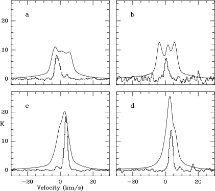
![\begin{figure}\includegraphics[width=11cm]{h1787f4.eps} \end{figure}](/articles/aas/full/2000/10/h1787/img51.gif) |
Figure 4:
The same as Fig. 3 for the 12CO(2-1)
emission in the central part of MBM 32 observed with the MRS at a
2 |
The line widths of the negative velocity cloud (and possibly also of the weak
emission in the interval 0 - 2 km s-1) are somewhat larger than those of
the main cloud. This is consistent with the findings of de Vries et al.
([1987]). Within the main cloud, line widths at the west side
(
![]()
![]() )
are significantly smaller than in the rest of the
cloud. This is
seen in all transitions, but the effect depends on the velocity resolution of
the different spectra. The 115 GHz HRS data show an average value of
1.12
)
are significantly smaller than in the rest of the
cloud. This is
seen in all transitions, but the effect depends on the velocity resolution of
the different spectra. The 115 GHz HRS data show an average value of
1.12 ![]() 0.26 km s-1 (135 positions) in the western part and of
1.49
0.26 km s-1 (135 positions) in the western part and of
1.49 ![]() 0.33 (249
positions) in the eastern part. This division is not clearly correlated with
some clumps or peaks in the cloud. The negative velocity emission has an
average line width of 1.92
0.33 (249
positions) in the eastern part. This division is not clearly correlated with
some clumps or peaks in the cloud. The negative velocity emission has an
average line width of 1.92 ![]() 0.63 km s-1 (108 positions). Except for the
region NE of (7
0.63 km s-1 (108 positions). Except for the
region NE of (7![]() , 21
, 21![]() )
(see above), the differences in line widths
cannot be explained by the presence of more than one velocity component along
the line of sight.
)
(see above), the differences in line widths
cannot be explained by the presence of more than one velocity component along
the line of sight.
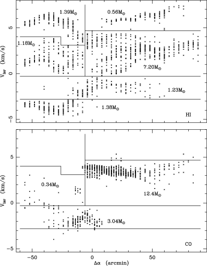
Because the H I emission has a larger velocity range and intrinsic
line width than the CO emission (see Fig. 5), and shows small
differences in velocity compared
to the CO (see below), it is not much of use to integrate the H I
emission over the same velocity interval as the CO or to investigate the peak
intensities. Instead we show in Fig. 6 the channel maps with
intervals of 2 km s-1 between -8 and +10 km s-1. H I at
negative velocities is mainly present in the western part of the cloud where
there is also CO emission at
![]() km
km![]() s-1. The main part
of the H I emission is in the interval
+1 to +4 km s-1 where there is some correlation of the H I
distribution with that of the strongest CO component. The strongest H I
is just NE of the eastern CO peak.
The negative velocity CO component, which it's approximately elliptical
distribution shows a similar structure in H I at
-4 to -2 km
s-1. The main part
of the H I emission is in the interval
+1 to +4 km s-1 where there is some correlation of the H I
distribution with that of the strongest CO component. The strongest H I
is just NE of the eastern CO peak.
The negative velocity CO component, which it's approximately elliptical
distribution shows a similar structure in H I at
-4 to -2 km![]() s-1 and -2 to 0 km
s-1 and -2 to 0 km![]() s-1
which seems to be slightly outside the CO emission region.
s-1
which seems to be slightly outside the CO emission region.
The velocity structure of the H I gas associated with MBM 32 is
shown from another perspective in Fig. 7, which contains position
(
![]() )
- velocity diagrams at
)
- velocity diagrams at ![]() -offsets from -24
-offsets from -24![]() to +44
to +44![]() .
The velocity components from Fig. 5 are clearly
visible, along with many other structures, such as secondary maxima, holes,
and velocity gradients, which cannot easily be modeled.
.
The velocity components from Fig. 5 are clearly
visible, along with many other structures, such as secondary maxima, holes,
and velocity gradients, which cannot easily be modeled.
We have made Gaussian fits to the H I spectra using two to four velocity
components: one weak (few K) and broad (typically 20 -
40 km![]() s-1) component and stronger but narrower (<10 km
s-1) component and stronger but narrower (<10 km![]() s-1)
components. The broad component shows little variation in intensity over the
mapped region and we assume that it is not associated with MBM 32. In
Fig. 8 we compare the velocities of the narrow components with
the
s-1)
components. The broad component shows little variation in intensity over the
mapped region and we assume that it is not associated with MBM 32. In
Fig. 8 we compare the velocities of the narrow components with
the
![]() of the MRS+HRS 12CO(1-0) data. Only in part of the
main CO cloud (-5
of the MRS+HRS 12CO(1-0) data. Only in part of the
main CO cloud (-5![]()
![]()
![]() )
the velocities of
one of the H I components agrees with the CO velocities within
0.5 km
)
the velocities of
one of the H I components agrees with the CO velocities within
0.5 km![]() s-1. For the other CO components differences are in the range
-1.5 - +1.5 km
s-1. For the other CO components differences are in the range
-1.5 - +1.5 km![]() s-1. At positions where there are such differences,
the H I spectra do not show signs of self absorption due to cold
foreground gas. These differences are less than the velocity dispersion of the
molecular gas: the line widths of spectra of the sum of all 12CO(1-0)
MRS data are 2.4 km
s-1. At positions where there are such differences,
the H I spectra do not show signs of self absorption due to cold
foreground gas. These differences are less than the velocity dispersion of the
molecular gas: the line widths of spectra of the sum of all 12CO(1-0)
MRS data are 2.4 km![]() s-1 (main component) and 3.4 km
s-1 (main component) and 3.4 km![]() s-1(negative velocity component). It is possible that only the H I gas in a
certain velocity range is converted into H2, leaving stronger emission at
higher or lower velocities. Or H I at one edge of the cloud has a
different velocity due to external pressure. H I line widths of all
components are about
4 - 5 km
s-1(negative velocity component). It is possible that only the H I gas in a
certain velocity range is converted into H2, leaving stronger emission at
higher or lower velocities. Or H I at one edge of the cloud has a
different velocity due to external pressure. H I line widths of all
components are about
4 - 5 km![]() s-1: the average value for the component associated with the main CO
cloud is 4.95
s-1: the average value for the component associated with the main CO
cloud is 4.95 ![]() 1.98 km
1.98 km![]() s-1; those of the three components at negative
offsets are 4.35
s-1; those of the three components at negative
offsets are 4.35 ![]() 0.91 km
0.91 km![]() s-1 (
s-1 (
![]() km
km![]() s-1), 4.75
s-1), 4.75 ![]() 1.75 km
1.75 km![]() s-1(
s-1(
![]() km
km![]() s-1), and 4.31
s-1), and 4.31 ![]() 1.20 km
1.20 km![]() s-1 (
s-1 (
![]() km
km![]() s-1).
These values are a factor 2 - 4 larger than the CO line widths in the same
region, which is less than expected from the difference in mass of H I
and CO.
It suggests that either the molecular gas is relatively more turbulent, or
the H I gas is colder. We have used the H I data to derive masses
assuming the emission is optically thin
[N(H I) =
s-1).
These values are a factor 2 - 4 larger than the CO line widths in the same
region, which is less than expected from the difference in mass of H I
and CO.
It suggests that either the molecular gas is relatively more turbulent, or
the H I gas is colder. We have used the H I data to derive masses
assuming the emission is optically thin
[N(H I) =
![]() dv cm-2].
The resulting values (not including He) are
indicated in Fig. 8 for the different velocity components. We also
indicate the H2 masses derived from CO (see Sect. 4.1). If all H I is
associated with MBM 32, both masses are approximately equal for the main CO
component. For the negative velocity component, the H2 mass is somewhat
larger than the H I mass (however this depends which region is
considered).
dv cm-2].
The resulting values (not including He) are
indicated in Fig. 8 for the different velocity components. We also
indicate the H2 masses derived from CO (see Sect. 4.1). If all H I is
associated with MBM 32, both masses are approximately equal for the main CO
component. For the negative velocity component, the H2 mass is somewhat
larger than the H I mass (however this depends which region is
considered).
![\begin{figure}\includegraphics[width=11cm]{h1787f6.eps} \end{figure}](/articles/aas/full/2000/10/h1787/img61.gif) |
Figure 6: Channel maps of H I emission in intervals of 2 km s-1 between -8 and 10 km s-1. Contour levels are 6 to 60 K km s-1 in steps of 6 K km s-1. For comparison in the upper left panel the 12CO(1-0) distribution for the three velocity intervals from Fig. 1, as grey-scale (Fig. 1s), full-drawn (Fig. 1b), and as dotted (Fig. 1c) contours |
Before we can compare the CO, H I, and FIR emission, we have to
convolve the CO and IRAS 60 and 100 ![]() m data first to the same resolution
as the H I (9
m data first to the same resolution
as the H I (9
![]() 2) data. Here we use only the 12CO(1-0) MRS map
because it covers the largest area on the sky. Subsequently we sampled the
FIR data at the same (4
2) data. Here we use only the 12CO(1-0) MRS map
because it covers the largest area on the sky. Subsequently we sampled the
FIR data at the same (4![]() )
raster
as both other data sets. The correlation between FIR and H I emission was
investigated by selecting positions where the convolved CO spectra showed
no emission stronger than about 0.2 K (114 positions). We compared
the 100
)
raster
as both other data sets. The correlation between FIR and H I emission was
investigated by selecting positions where the convolved CO spectra showed
no emission stronger than about 0.2 K (114 positions). We compared
the 100 ![]() m emission with the H I emission integrated over the whole
velocity range where there is emission (-80 to 50 km
m emission with the H I emission integrated over the whole
velocity range where there is emission (-80 to 50 km![]() s-1), with the
H I
emission of the narrow components in the Gaussfits, and with all the local
emission (including the broad component).
It appears (using the bisector linear least squares fit, see Isobe et al.
[1990])
that in the latter case the correlation is best (correlation coefficient 0.60),
however the offset remains rather uncertain:
s-1), with the
H I
emission of the narrow components in the Gaussfits, and with all the local
emission (including the broad component).
It appears (using the bisector linear least squares fit, see Isobe et al.
[1990])
that in the latter case the correlation is best (correlation coefficient 0.60),
however the offset remains rather uncertain:
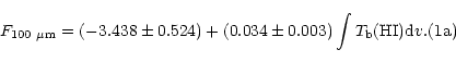
The results (Eq. 1) were used to correct the FIR emission for dust associated
with H I towards the 403 positions where there is CO emission, and
subsequently we obtained the following relation between 100 ![]() m emission and
12CO(1-0) integrated line intensities:
m emission and
12CO(1-0) integrated line intensities:
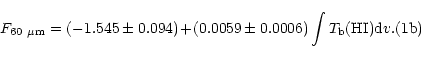
For 60 ![]() m our result is (correlation coefficient 0.60):
m our result is (correlation coefficient 0.60):
The slope in Eq. (1a) translates into a ratio of H I column density
and 100 ![]() m flux density of
N(H)/
m flux density of
N(H)/
![]() cm-2 Jy-1 sr. Comparing this
with Eq. (2) of Meyerdierks & Heithausen ([1996]) we find that the
cm-2 Jy-1 sr. Comparing this
with Eq. (2) of Meyerdierks & Heithausen ([1996]) we find that the
![]() m emission per H atom is a factor 2.6 smaller in MBM 32 than in the
Polaris Flare.
m emission per H atom is a factor 2.6 smaller in MBM 32 than in the
Polaris Flare.
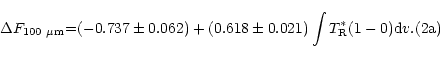
The slope in Eq. (2a), 0.618 MJy s (K km sr)-1 is slightly steeper than
the value found by Meyerdierks & Heithausen [0.5 MJy s (K km sr)-1].
However their Fig. 7 essentially shows a scatterplot and no accurate
value for the slope could be determined. From Eqs. (1a) and (2a) we obtain
a conversion factor between
![]() CO(1-0))
and N(H2) of
(0.17
CO(1-0))
and N(H2) of
(0.17 ![]()
![]() cm-2 (K km s
-1)-1, much lower
than derived from our CO data alone (
cm-2 (K km s
-1)-1, much lower
than derived from our CO data alone (
![]() ;
see Sect. 4.1), but similar to values
derived in the same way towards some parts of the Draco nebula by
Herbstmeier et al. ([1993]). However, this value is a lower limit
(possibly by a factor 2 or 3) if the dust temperature is lower in the inner
parts of the cloud (see Meyerdierks & Heithausen [1996]).
;
see Sect. 4.1), but similar to values
derived in the same way towards some parts of the Draco nebula by
Herbstmeier et al. ([1993]). However, this value is a lower limit
(possibly by a factor 2 or 3) if the dust temperature is lower in the inner
parts of the cloud (see Meyerdierks & Heithausen [1996]).
Our results can also be used to derive the dust temperature and mass. A
correlation between 60 and 100 ![]() m emission associated with MBM 32 gives
(correlation coefficient 0.92):
m emission associated with MBM 32 gives
(correlation coefficient 0.92):
Copyright The European Southern Observatory (ESO)
![\begin{figure}\includegraphics[width=9cm]{h1787f3.eps} \end{figure}](/articles/aas/full/2000/10/h1787/img49.gif)
![\begin{figure}\includegraphics[width=11cm]{h1787f7.eps} \end{figure}](/articles/aas/full/2000/10/h1787/img62.gif)