)
)
The Si:Ga linear detector of the PHT-S channel of ISOPHOT has been
extensively studied by
Fouks and Schubert from experimental and theoretical points of view
(Fouks 1992; Schubert et al. 1994; Fouks & Schubert 1995;
Schubert et al. 1995; Schubert 1995). The LW ISOCAM detector is a Si:Ga
array too. Its size is 32  32 pixels, 100
  m pitch and the thickness of
500 m.
PHT-S pixels size are 0.35
0.37 mm (for 64 pixels long)
and the thickness is 2.0 mm.
Wavelength ranges are 6.-12. m for PHT-S
and 4.-17. m for LW ISOCAM.
m pitch and the thickness of
500 m.
PHT-S pixels size are 0.35
0.37 mm (for 64 pixels long)
and the thickness is 2.0 mm.
Wavelength ranges are 6.-12. m for PHT-S
and 4.-17. m for LW ISOCAM.
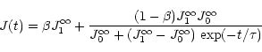
In this paper, we will not describe the semi conductor physics equations but only indicate the more relevant references. Because of the intrinsic non linear nature of the equations and of the sensitivity to the boundary conditions, several steps were needed from the first linearized solutions (Suris & Fouks 1978; Suris & Fouks 1980) to the final non linear solutions covering a large range of detectors (Vinokurov & Fouks 1991; Fouks 1992). For the detectors of PHT-S and LW-ISOCAM, the most relevant paper to understand the physics is Fouks & Schubert (1995). It is based on the first order description of the physics inside the bulk of an extrinsic p-type photo-conductor. After several hypothesis about the dominant physical processes, a set of conditions and differential equations is obtained. Solving the set of differential equations assuming a constant electric field inside the bulk, a Riccati differential equation is found. Its solution which gives the temporal response is a non linear equation.
The first solution describes the response to a instantaneous
step of flux at time t=0, from the constant level
 to the constant level
 :
:
is the stabilized photo-current measured at time
 .
It is also directly related to the observed flux, since
a linear relationship is assumed between the flux and the photo-current
after stabilization (Fouks & Schubert 1995).
The parameter
.
It is also directly related to the observed flux, since
a linear relationship is assumed between the flux and the photo-current
after stabilization (Fouks & Schubert 1995).
The parameter  characterizes the instantaneous jump just after the
flux change. The theory gives
a simple relationship between the time constant
characterizes the instantaneous jump just after the
flux change. The theory gives
a simple relationship between the time constant  and
over several order of magnitude:
and
over several order of magnitude:
 .
Yet, the time constant is
.
Yet, the time constant is  .
This dependence has also been observed for the LW channel of ISOCAM
(Sect. 3.4 and Abergel et al. 1999).
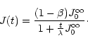
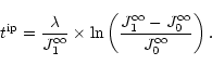
Equation (1) does not allow us to compute J(t)if
.
This dependence has also been observed for the LW channel of ISOCAM
(Sect. 3.4 and Abergel et al. 1999).
Equation (1) does not allow us to compute J(t)if
 ,
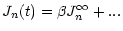
and for that case a first order development gives:
,
and for that case a first order development gives:
On data (ground based and in-flight data),
starting from a level close to the dark level
(lower than 1 ADU/G/s), an inflection point (see Sect. 2
and Fig. 2) is clearly visible for moderate upward steps
(typically above 10 ADU/G/s and below 100 ADU/G/s).
It is more difficult to observe it
for strong upward steps since it is temporally very close to the jump.
No inflection point is visible for small upward steps
(ratio
 between 1 and 2)
and for downward steps.
This inflection point is predicted and perfectly reproduced with
Eq. (1). Its position
between 1 and 2)
and for downward steps.
This inflection point is predicted and perfectly reproduced with
Eq. (1). Its position
 can be easily calculated from
Eq. (1). For
can be easily calculated from
Eq. (1). For
 ,
we obtain:
,
we obtain:
 ).
The inflection point appears for upwards steps only
when
).
The inflection point appears for upwards steps only
when
 .
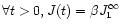
For
.
For
 ,
,
 ,
so in that case
the response is constant and,
,
so in that case
the response is constant and,
 .
However the case
strictly equal to 0 (and obviously
.
However the case
strictly equal to 0 (and obviously
 )
is not physical,
since the detector always receives infrared photons due to thermal emissions
of the different parts of the camera (even when it is switched off).
For
,
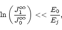
Fig. 4
illustrates the variations of the position of
the inflection point with the value of the initial level J0.
)
is not physical,
since the detector always receives infrared photons due to thermal emissions
of the different parts of the camera (even when it is switched off).
For
,
Fig. 4
illustrates the variations of the position of
the inflection point with the value of the initial level J0.
![\begin{figure}\par\includegraphics[angle=90,width=8.5cm]{ds8869f4.eps}
\par\end{figure}](/articles/aas/full/2000/03/ds8869/img46.gif) |
Figure 4:
FS model response to upward and downward steps of flux,
from Eq. (1) (see also Fig. 8 in Schubert & Fouks
1995). Upward steps of flux from a constant level J0to a constant level J1 occur at time t=100 s and downward
steps from J1 to J0 at t=900 s. We have taken:
J0 = 0.01, 0.1, 1.0, 2.0 and 5.0 ADU/G/s, and J1= 10 ADU/G/s.
For all these simulations, the values of the parameters
and
are constant.
We see that Eq. (1) is very sensitive
to the initial level (J0) for the upward steps:
curves from 0.01, 0.1 and 1.0 ADU/G/s are very different.
When the dark level is poorly estimated,
such non linear effect can allow us to correct the value of J0 |
Equation (1) can only be used for transitions between stabilized levels.
The following enhancement (Fouks & Schubert 1995) allows us to
describe a not stabilized detector output J n(t) from
a recursive point of view (see Fig. 5 for notations).
An observation is made of N integrations starting at time tn.
We assume that the input flux
 is
constant during each successive integration.
During the integration number n, we have:
is
constant during each successive integration.
During the integration number n, we have:
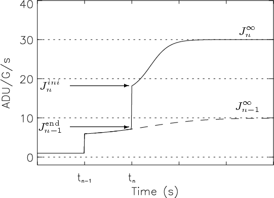 |
Figure 5:
Response to two successive upward steps of flux
(at time tn-1 = 100 s and tn = 200 s
respectively), corresponding to three blocks of constant input fluxes
(number n-2, n-1 and n respectively). We have taken
= 0.55,
= 600. ADU/G,
 = 1. ADU/G/s,
 = 10. ADU/G/s and
= 30. ADU/G/s.
This figure is adapted from Fouks & Schubert (1995)
= 10. ADU/G/s and
= 30. ADU/G/s.
This figure is adapted from Fouks & Schubert (1995) |
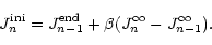
Basically we use the same notations as in Eq. (1).
 is the response measured
just after the jump at time tn.
J n(t) is the response at any time t between tn and tn+1.
In this equation, the state at the end of the previous integration n-1 is
contained in
,
which can be related
to the previous flux and the current stabilized flux values
(
and
)
and the final previous flux just before the jump
is the response measured
just after the jump at time tn.
J n(t) is the response at any time t between tn and tn+1.
In this equation, the state at the end of the previous integration n-1 is
contained in
,
which can be related
to the previous flux and the current stabilized flux values
(
and
)
and the final previous flux just before the jump
 by:
by:
Finally, we obtain from Eq. (4) and Eq. (5):
,
and
(Fig. 5).
If we take:
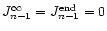 ,
we have
,
we have
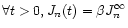 ,
and
,
and
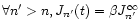 .
Negative values for
are not physical
and would give, after the instantaneous jump, a monotonous decrease
with a vertical asymptote located after the jump
(its position can be calculated from Eq. (1)).
.
Negative values for
are not physical
and would give, after the instantaneous jump, a monotonous decrease
with a vertical asymptote located after the jump
(its position can be calculated from Eq. (1)).
We have adjusted the model of the response on experimental data,
both on the averaged response within the 1111 central
square and for individual pixels.
We have used data with limited flux steps, since
the response for steps greater than  150 ADU/G/s is
too fast to give accurate values (typically a few integrations).
150 ADU/G/s is
too fast to give accurate values (typically a few integrations).
We illustrate the results with data already
presented in Sect. 2.
The signal was stabilized before the flux changes.
The values
and
are known.
We have three free parameters to fit Eq. (1)
with the data, the two parameters
and ,
and an offset level.
To add an offset is mandatory for some observations
(especially for the ground base data) since the absolute dark level was
poorly estimated while the response is
very sensitive to the initial level before the flux step,
therefore to the absolute value of the dark level
(see Sect. 3.2 and Fig. 4).
The three parameters are adjusted by least square fitting
( criterion with constant error).
We see on the examples we present (Figs. 2
and 3) that the model remarkably reproduces
both upward and downward steps. Other steps have been adjusted,
with higher and lower amplitudes, with a similar accuracy.
Especially, the position of the inflection point of upward steps is
accurately reproduced.
criterion with constant error).
We see on the examples we present (Figs. 2
and 3) that the model remarkably reproduces
both upward and downward steps. Other steps have been adjusted,
with higher and lower amplitudes, with a similar accuracy.
Especially, the position of the inflection point of upward steps is
accurately reproduced.
We have also made adjustments when the signal was not stabilized before
the changes of flux using Eq. (6) to estimate
the value of  for each block
(one block corresponding to a constant configuration of the whole system,
see Sect. 4).
We assume that
and
are constant
over the whole observation. We see in Fig. 6 that the
precision is
for each block
(one block corresponding to a constant configuration of the whole system,
see Sect. 4).
We assume that
and
are constant
over the whole observation. We see in Fig. 6 that the
precision is  .
We have the same kind of results for different datasets taken
during the whole life of the satellite. We have also
checked that the theoretical relationship
.
We have the same kind of results for different datasets taken
during the whole life of the satellite. We have also
checked that the theoretical relationship
 predicted by Suris & Fouks (1980) is verified by the data,
for uniform illumination of the detector and for upward and downward steps
of flux in the range of a few ADU/G/s to
500 ADU/G/s.
predicted by Suris & Fouks (1980) is verified by the data,
for uniform illumination of the detector and for upward and downward steps
of flux in the range of a few ADU/G/s to
500 ADU/G/s.
)
The fitting method described in the previous section has been applied for the
32
32 pixels of the detector in order to derive for each pixel the
values of
and
for uniform illumination.
Practically, we have used long-term observations
of the zodiacal background taken successively with two filters.
First the data have been dark corrected, then glitches have been removed
using a temporal median filtering which detect all pixels deviating from the
running median value by more than a threshold value.
In order to remove glitches still contained in the data
(especially those with significant memory effects, Désert 1999),
two pass fitting is used. For the second pass, pixels deviating
from the running averaged value of more than 3 are discarded.
The correction of glitches with negative tail is much more
difficult and manual removing is necessary for a limited number of case.
In any case, this two pass fitting does not discard all glitches with memory
effects.
are discarded.
The correction of glitches with negative tail is much more
difficult and manual removing is necessary for a limited number of case.
In any case, this two pass fitting does not discard all glitches with memory
effects.
The FS model is not symmetrical. The adjustment of
and is more accurate for upward steps than downward steps,
because the
values present in the (
)
plane
a steeper minimal value for upward steps than downward steps.
On simulated noisy data, we have obtained a precision
of
 and
and
 for upward steps, and only
 and
and
 for downward steps.
We have used upward steps of flux on quasi uniform illumination
(essentially zodiacal emission)
with
from 5 to 25 ADU/G/s and
a ratio
in the range 2-5.
This range is unfortunately limited for in-flight data
by the zodiacal emission characteristics.
Values of
lower than 10 ADU/G/s give poor adjustments,
likely due to uncertainties in the dark level.
Actually, six independent data sets (from scientific observations
of diffuse clouds taken during revolutions
number 129, 321, 590, 658, 684 and 772) have been extensively analyzed.
Because of (1) glitches with memory effects, (2) oscillations
in the response curve and (3) in some cases
low signals at the edge of the detector due to the optical vignetting,
the values of
and
cannot be
accurately estimated for typically  of the pixels in an observation. About 5 to 10
 of the pixels in each data set present oscillations
during the stabilization after the upward steps.
Most of these pixels are close to the edges or the corners of the
detector (Abergel et al. 1999). The FS model cannot describe such behavior, and
only
can be accurately estimated.
These oscillations will be discussed in Sect. 5.6.
of the pixels in each data set present oscillations
during the stabilization after the upward steps.
Most of these pixels are close to the edges or the corners of the
detector (Abergel et al. 1999). The FS model cannot describe such behavior, and
only
can be accurately estimated.
These oscillations will be discussed in Sect. 5.6.
We have computed six independent maps of
and from the six data sets we use.
On these maps, we have pixel to pixel variations which are significant.
They are reproducible on the six independent data sets.
The final maps of
and
are obtained
by averaging the six maps taking into account
for each pixel the
value for each data set
and discarding values by
clipping.
The final values of
have an absolute accuracy better
than  0.02 for 95
of the pixels.
For the final values of ,
the accuracy is better
than 20 ADU/G for 50
of the pixels
(the lower left part of the map presented in Fig. 7),
while for 10
of the pixels the accuracy is above 50 ADU/G.
The final maps are presented in Fig. 7,
compared to the map of the spatial variation of the response
for uniform illumination (the flat field).
Histograms are plotted in Fig. 8.
0.02 for 95
of the pixels.
For the final values of ,
the accuracy is better
than 20 ADU/G for 50
of the pixels
(the lower left part of the map presented in Fig. 7),
while for 10
of the pixels the accuracy is above 50 ADU/G.
The final maps are presented in Fig. 7,
compared to the map of the spatial variation of the response
for uniform illumination (the flat field).
Histograms are plotted in Fig. 8.
![\begin{figure}\par\includegraphics[width=8.5cm]{ds8869f8.eps}
\par\end{figure}](/articles/aas/full/2000/03/ds8869/img69.gif) |
Figure 8:
Histogram of
(upper panel) and
(lower panel)
for the 32
32 pixels and from data of Fig. 7 |
The accuracy on the final maps of
and
is limited because
(1) only six data sets have been used with a limited range
of the
ratio,
(2) at low
ratio
the FS model is not very sensitive to ,
(3) several pixels are affected by glitches,
(4) for some pixels only one or two
independent values have been used
and (5) uncertainties in the dark level.
The mean values of
and
are equal to
 = 0.51 and
 = 560 ADU/G.
The data taken during the ground-based tests have also been extensively
used to explore the transient behavior over a wide dynamic range.
Different values (
= 560 ADU/G.
The data taken during the ground-based tests have also been extensively
used to explore the transient behavior over a wide dynamic range.
Different values (
 0.6 and
 400 ADU/G) are obtained
due to a different setup of the detector.
400 ADU/G) are obtained
due to a different setup of the detector.
One important assumption of the FS model is (Vinokurov & Fouks 1991):
and ,
since:
 V/m and
 V/m
then the condition 7 is satisfied.
For PHOT-S, Schubert (1995) indicates
V/m
then the condition 7 is satisfied.
For PHOT-S, Schubert (1995) indicates
 V/m and
 V/m.
V/m.
Copyright The European Southern Observatory (ESO)


![\begin{figure}\par\includegraphics[angle=90,width=8.5cm]{ds8869f6.eps}
\par\end{figure}](/articles/aas/full/2000/03/ds8869/img57.gif)
![\begin{figure}\par\includegraphics[width=7.8cm]{ds8869f7a.eps}
\includegraphics[...
...cm]{ds8869f7b.eps}
\includegraphics[width=7.8cm]{ds8869f7c.eps}
\par\end{figure}](/articles/aas/full/2000/03/ds8869/img62.gif)