In this appendix, we will clarify the question under which circumstances the
local slope of (generalized) line-strength distribution functions can be
equalized to the CAK force multiplier ![]() .
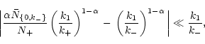
Following
Eq. (24) in Sect. 2.3.2, this is possible under the condition
.
Following
Eq. (24) in Sect. 2.3.2, this is possible under the condition
| |
Figure A1:
Schematic sketch of two different kinds of line-number
distributions, case A (left) and B (right). Note the log-log representation
necessary to derive the local slope |
which depends strongly on the average cumulative line number
![]() (cf.
Eq. 25). To proceed further, we have to investigate two cases.
Case A, which is the more realistic one (cf. Sect. 4), comprises a
situation where the line-number distribution has a monotonic curvature in
the log, corresponding to an increase of
(cf.
Eq. 25). To proceed further, we have to investigate two cases.
Case A, which is the more realistic one (cf. Sect. 4), comprises a
situation where the line-number distribution has a monotonic curvature in
the log, corresponding to an increase of ![]() for decreasing
for decreasing ![]() .
This
situation is sketched on the left of Fig. A1: Both the total line
number N(0) (as well as
.
This
situation is sketched on the left of Fig. A1: Both the total line
number N(0) (as well as
![]() denoted by N0 in our plots)
and the average number of lines
denoted by N0 in our plots)
and the average number of lines
![]() lie well below the extrapolated value
lie well below the extrapolated value
![]() .
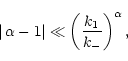
In this case, it is straightforward to show that the lhs of
(A1) obtains its maximum value for the smallest value possible for
.
In this case, it is straightforward to show that the lhs of
(A1) obtains its maximum value for the smallest value possible for
![]() ,
which is N-. Using this value, the inequality becomes
,
which is N-. Using this value, the inequality becomes
which under the considered circumstances can be (almost) always fulfilled as
long as
![]() ! Thus, for monotonically curved but otherwise
unconstrained
! Thus, for monotonically curved but otherwise
unconstrained
![]() distributions (case A), the ensemble line
acceleration follows the local (however not necessarily constant)
slope of the flux-weighted and cumulative line-strength distribution
function, as long as this is larger than -1.
distributions (case A), the ensemble line
acceleration follows the local (however not necessarily constant)
slope of the flux-weighted and cumulative line-strength distribution
function, as long as this is larger than -1.
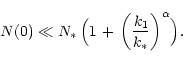
Case B (right panel of Fig. A1) displays the situation of a
sharply increasing line number below a certain threshold value k*. The
asymptotic fit value ![]() is here significantly smaller than the
actual value N(0) and the average value
is here significantly smaller than the
actual value N(0) and the average value
![]() .
In this case, we define
N* as the number of lines where the actual distribution and the fitted
one cross each other, at line-strength k*. To obtain an upper limit for
our inequality (A1), we use the maximum possible value for
.
In this case, we define
N* as the number of lines where the actual distribution and the fitted
one cross each other, at line-strength k*. To obtain an upper limit for
our inequality (A1), we use the maximum possible value for
![]() ,
,
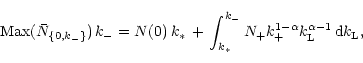
which after some algebra leads to the requirement
 |
(A3) |
This requirement can be usually fulfilled if ![]() is large compared
to k* (i.e., the sharp increase of line number occurs at relatively
small line-strength), and, again, if
is large compared
to k* (i.e., the sharp increase of line number occurs at relatively
small line-strength), and, again, if ![]() is positive.
is positive.
In summary, we have shown that the CAK representation
![]() with
with ![]() corresponding to the local slope of the
line-strength distribution function is valid under fairly general
circumstances, if the slope is not too steep in the region around
corresponding to the local slope of the
line-strength distribution function is valid under fairly general
circumstances, if the slope is not too steep in the region around ![]() ,
i.e.,
,
i.e.,
![]() locally. Of course, if the distribution function is
curved, this leads immediately to depth dependent force-multiplier
parameters.
locally. Of course, if the distribution function is
curved, this leads immediately to depth dependent force-multiplier
parameters.
Finally, it is important to realize that our derivation has required some
knowledge of the behaviour of optically thin lines, however did not
constrain the distribution of optically thick lines in any respect. This, of
course, is related to the fact that all optically thick lines behave
similarly. Thus, the slope of the distribution for
![]() is of no
concern as long as we know the actual number of these lines.
is of no
concern as long as we know the actual number of these lines.
Copyright The European Southern Observatory (ESO)