In this appendix, we give a brief derivation of the frequency integrated
line intensity distribution function, Eq. (73). Similar to the
frequency dependent one, Eq. (61), which is the
starting point of our considerations, we have to account for different regimes,
since the maximum possible (logarithmic) oscillator strength
![]() depends
both on line intensity and frequency. Furthermore, we assume that under
certain circumstances only levels below a cutoff
depends
both on line intensity and frequency. Furthermore, we assume that under
certain circumstances only levels below a cutoff
![]() shall contribute.
In this case then, all lines with lower levels energetically higher than
shall contribute.
In this case then, all lines with lower levels energetically higher than
![]() are neglected. This generalization will turn out to be important if
NLTE-effects are included into our approach (cf. Sect. 4.2.3).
are neglected. This generalization will turn out to be important if
NLTE-effects are included into our approach (cf. Sect. 4.2.3).
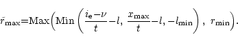
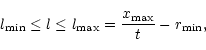
Finally, we allow for an integration between
![]() ,
since
for high ionization energies our line list may be incomplete (and
useless, if one accounts for the vanishing flux) beyond a certain maximum
frequency.
,
since
for high ionization energies our line list may be incomplete (and
useless, if one accounts for the vanishing flux) beyond a certain maximum
frequency.
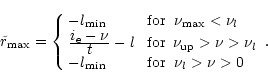
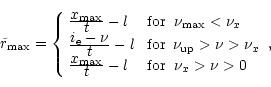
At first note, that the maximum possible oscillator strength is given by
| (E2) |
At low line intensities,
![]() ,
we have to
account for the minimum
,
we have to
account for the minimum
![]() ,
which introduces a threshold frequency
,
which introduces a threshold frequency
![]() :
:
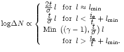
By integrating Eq. (61) over frequency and accounting for these
different cases (four in total), we finally obtain the following expressions
for the function F defined in Eq. (73).
| = | |||
| = | |||
| = | |||
| = | |||
| = |
The most important fact concerning the derived function is the following:
Depending on line intensity and the specific value of A, the distribution
can show three different slopes, namely
![]() and
and
![]() ,
where the first one and the last have been found already for
the frequency dependent distribution function (cf. Sect. 4.2.1), whereas the
second one is a new feature arising from the frequency integration.
,
where the first one and the last have been found already for
the frequency dependent distribution function (cf. Sect. 4.2.1), whereas the
second one is a new feature arising from the frequency integration.
Let us briefly consider under which condition which slope will show up. At
first, assume that
![]() ,
i.e., both the level list and the
line list shall be complete. In this case, Eqs. (E7) and
(E9) have to be applied (
,
i.e., both the level list and the
line list shall be complete. In this case, Eqs. (E7) and
(E9) have to be applied (![]() ).
).
For (very) low line intensities, l is approximately
![]() and
and
![]() .
Thus, the second term in (E7) dominates
and the result is similar to (E6), with maximum frequency
.
Thus, the second term in (E7) dominates
and the result is similar to (E6), with maximum frequency ![]() .
In
consequence, F is independent on l and the apparent slope of the
distribution is
.
In
consequence, F is independent on l and the apparent slope of the
distribution is ![]() (remember, that
(remember, that
![]() ). In this situation, for (almost) all possible line
frequencies the contributing oscillator strengths stretch from
). In this situation, for (almost) all possible line
frequencies the contributing oscillator strengths stretch from
![]() to
to
![]() .
.
For larger l then, ![]() decreases, whereas
decreases, whereas
![]() for l
being smaller than
for l
being smaller than
![]() .
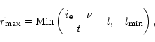
We encounter the case that the maximum possible
oscillator strength
.
We encounter the case that the maximum possible
oscillator strength
![]() can no longer be reached for large frequencies
(cf. Eq. (E4), middle panel), and the apparent slope is controlled by
the sign of A. For negative and not too small A, i.e.,
can no longer be reached for large frequencies
(cf. Eq. (E4), middle panel), and the apparent slope is controlled by
the sign of A. For negative and not too small A, i.e.,
![]() ,
,
| (E10) |
For positive A, i.e.,
![]() ,
the situation is different. Now the
first bracket of (E7) dominates, giving rise (via the combination
of exponents
,
the situation is different. Now the
first bracket of (E7) dominates, giving rise (via the combination
of exponents
![]() )
to an exact
slope of
)
to an exact
slope of ![]() ,
since the dependence on
,
since the dependence on ![]() cancels completely.
This behaviour is finally reached also for negative A and larger l:
For
cancels completely.
This behaviour is finally reached also for negative A and larger l:
For
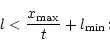
![]() ,
the upper frequential boundary
,
the upper frequential boundary
![]() is
is ![]() ,
which
has the same dependency on l as
,
which
has the same dependency on l as ![]() .
Additionally, the impact of
small oscillator strengths becomes smaller, simply because the last term in
(E6) decreases with
.
Additionally, the impact of
small oscillator strengths becomes smaller, simply because the last term in
(E6) decreases with ![]() as function of l.
as function of l.
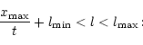
Nothing changes for negative A and even larger l, when Eq. (E9)
applies. The slope remains at its value ![]() .
For positive A,
however, there is a dramatic change for
.
For positive A,
however, there is a dramatic change for
![]() .
Due to the
interrelation of line intensity and
.
Due to the
interrelation of line intensity and
![]() (cf. the discussion in Sect. 4.2.1),
the dependence on
(cf. the discussion in Sect. 4.2.1),
the dependence on ![]() cancels and only the
cancels and only the
![]() slope
survives (the 2nd term in (E9) being now the dominating one). Thus
for
slope
survives (the 2nd term in (E9) being now the dominating one). Thus
for ![]() (well) below
(well) below
![]() the apparent slope at high line intensities
is coupled to the oscillator strength statistics. Finally if
the apparent slope at high line intensities
is coupled to the oscillator strength statistics. Finally if
![]() (corresponding to the case A=0 which cannot be treated by the
above formalism), it turns out that the slope at large l
smoothly changes from
(corresponding to the case A=0 which cannot be treated by the
above formalism), it turns out that the slope at large l
smoothly changes from
![]() to
to ![]() .
.
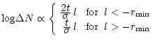
In summary, we have the following behaviour of ![]() if
if
![]() :
:
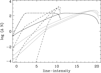
We have considered two case, namely
![]() and 0.93,
respectively, to demonstrate the dependence on
and 0.93,
respectively, to demonstrate the dependence on
![]() .
In the first case
then,
.
In the first case
then,
![]() = 1.46, and the fully drawn line (
= 1.46, and the fully drawn line (
![]() )
and the
dotted ones
)
and the
dotted ones
![]() display the resulting distribution
functions. As predicted by Eq. (E12), the curve for
display the resulting distribution
functions. As predicted by Eq. (E12), the curve for
![]() displays two effective slopes, namely
displays two effective slopes, namely ![]() and
and
![]() ,
where
the dividing line intensity is given by
,
where
the dividing line intensity is given by
![]() .
For
.
For
![]() ,
only one slope (
,
only one slope (![]() )
is present due to the third condition
in Eq. (E12). In contrast, the behaviour for
)
is present due to the third condition
in Eq. (E12). In contrast, the behaviour for
![]() and 3 (
and 3 (
![]() ,
Eq. (E11)) depends on
,
Eq. (E11)) depends on
![]() and
and ![]() ,
with a corresponding boundary at
,
with a corresponding boundary at
![]() in our example.
in our example.
For the larger value of ![]() with
with
![]() ,
we see the transition
of slope
,
we see the transition
of slope ![]() to
to ![]() at
at
![]() for the
curves with
for the
curves with
![]() (dashed-dotted),
(dashed-dotted),
![]() and 1.6 (dashed).
Only the case with
and 1.6 (dashed).
Only the case with
![]() reaches its asymptotic value of
reaches its asymptotic value of
![]() ,
where also the steeper slope of
,
where also the steeper slope of ![]() for
for
![]() is clearly visible.
is clearly visible.
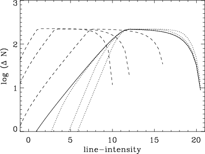 |
Figure E2:
Frequency integrated line intensity distribution function:
variation with
|
In Fig. E2 we demonstrate the influence of either varying the
highest energetic level (
![]() )
or the maximum line frequency (
)
or the maximum line frequency (
![]() ),
if all other parameters are kept constant. As long as
),
if all other parameters are kept constant. As long as
![]() (dotted curves), the only influence of decreasing
(dotted curves), the only influence of decreasing
![]() concerns the
region with
concerns the
region with
![]() ,
i.e., Eq. (E6) (partly) replaces
Eq. (E7), where the largest influence is close to
,
i.e., Eq. (E6) (partly) replaces
Eq. (E7), where the largest influence is close to
![]() .
Only for very
small values of
.
Only for very
small values of
![]() the complete first interval is affected. In
consequence, even for
the complete first interval is affected. In
consequence, even for
![]() the apparent slope becomes
the apparent slope becomes
![]() ,
since F depends no longer on l.
,
since F depends no longer on l.
In contrast, by diminishing
![]() while keeping
while keeping
![]() (dashed
curves), the slope of the first interval is barely affected, unless
(dashed
curves), the slope of the first interval is barely affected, unless
![]() becomes (very) small compared to
becomes (very) small compared to ![]() so that the transition value is close
to
so that the transition value is close
to
![]() (cf. E12, first panel). The major effect of decreasing
(cf. E12, first panel). The major effect of decreasing
![]() ,
however, is by shifting the dividing line (which is now a linear
function of
,
however, is by shifting the dividing line (which is now a linear
function of
![]() )
to smaller line intensities. Thus, a line-distribution
with
)
to smaller line intensities. Thus, a line-distribution
with
![]() different from
different from ![]() resembles the line-distribution of a
similar ion, however with much smaller ionization energy. This behaviour
turns out to be important if one considers the NLTE line-strength
statistics. Finally, if
resembles the line-distribution of a
similar ion, however with much smaller ionization energy. This behaviour
turns out to be important if one considers the NLTE line-strength
statistics. Finally, if
![]() approaches zero, the line distribution becomes independent on any excitation
effects. This limiting case, which corresponds to accounting for resonance
lines only, leads to a line-statistics influenced solely by the underlying
gf-distribution.
approaches zero, the line distribution becomes independent on any excitation
effects. This limiting case, which corresponds to accounting for resonance
lines only, leads to a line-statistics influenced solely by the underlying
gf-distribution.
 |
Figure E3:
Frequency integrated line intensity distribution function:
saturation effect. Basic parameters as in Fig. E2.
Fully drawn:
|
Figure E3 illustrates the effect of diminishing both
![]() and
and
![]() .
In principle, the effects are similar to the cases
studied above, namely the transition value is changed via
.
In principle, the effects are similar to the cases
studied above, namely the transition value is changed via
![]() ,
and the
slope of the first region increases to
,
and the
slope of the first region increases to ![]() .
However, there exists
another interesting effect, displayed by the dashed dotted curve: If the
maximum considered frequency
.
However, there exists
another interesting effect, displayed by the dashed dotted curve: If the
maximum considered frequency
![]() falls below the value of
falls below the value of
![]() ,
the distribution function becomes "saturated'', i.e., does no longer
change in shape (of course, the absolute value of F and thus the
total line number decreases with
,
the distribution function becomes "saturated'', i.e., does no longer
change in shape (of course, the absolute value of F and thus the
total line number decreases with
![]() ). The reason for this saturation
is given by the fact that Eqs. (E6) and (E8) now control the
behaviour of F, and that for
). The reason for this saturation
is given by the fact that Eqs. (E6) and (E8) now control the
behaviour of F, and that for
![]() this function depends on
this function depends on
![]() solely by a constant factor
solely by a constant factor
![]() for all
l.
for all
l.
Note, that in those cases when
![]() is small compared to
is small compared to ![]() (as is
typical under NLTE-conditions, see Sect. 4.2.3), this condition applies for
fairly large
(as is
typical under NLTE-conditions, see Sect. 4.2.3), this condition applies for
fairly large
![]() .
In other words: The shape of the
function is the same for all cutoff frequencies smaller than
.
In other words: The shape of the
function is the same for all cutoff frequencies smaller than
![]() :
At
maximum two slopes are present, namely either
:
At
maximum two slopes are present, namely either ![]() and
and ![]() for
for
![]() or
or ![]() for
for
![]() .
This fact
is essential for flux-weighted line-strength distribution function
(Sect. 4.2.8), since the maximum frequency which has to be considered for
this function is fairly small due to the decreasing flux at high energies.
.
This fact
is essential for flux-weighted line-strength distribution function
(Sect. 4.2.8), since the maximum frequency which has to be considered for
this function is fairly small due to the decreasing flux at high energies.
Acknowledgements
We like to thank Ken Gayley, Stan Owocki and Achim Feldmeier for useful comments and suggestions. This project has been supported in part by the Deutsche Forschungsgemeinschaft under DFG grants Pu 117-1/2 and Pa 477-1/2.
Copyright The European Southern Observatory (ESO)