Appendix B: The "À Trous'' wavelet transform algorithm

In a wavelet transform, a series of transformations of an image is generated, providing a resolution-related set of "views'' of the image. The properties satisfied by a wavelet transform, and in particular the à trous wavelet transform ("with holes'', so called because of the interlaced convolution used in successive levels: see step 2 of the algorithm below) are further discussed in (Starck et al. 1998).

We consider sampled data, $\{c_0(k)\}$, defined as the scalar product at pixels k of the function f(x) with a scaling function $\phi(x)$which corresponds to a low pass band filter:

$$c_0(k) = < f(x), \phi(x-k)\gt .$$ (17)

The scaling function is chosen to satisfy the dilation equation:

$$\frac{1}{2}\phi\left(\frac{x}{2}\right) = \sum_k h(k)\phi(x-k)$$ (18)

h is a discrete low pass filter associated with the scaling function $\phi$. This means that a low-pass filtering of the image is, by definition, closely linked to another resolution level of the image.

The smoothed data c_j(k) at a given resolution j and at a position k is the scalar product

$$c_j(k)= \frac{1}{2^j}< f(x), \phi\left(\frac{x-k}{2^j}\right)\gt.$$ (19)

This is consequently obtained by the convolution:

$$c_j(k) = \sum_l h(l) \ \ c_{j-1} (k+2^{j-1}l).$$ (20)

The signal difference w_j between two consecutive resolutions is:

w_j(k) = c_j-1(k) - c_j(k)

or:

$$w_j(k) = \frac{1}{2^j}< f(x), \psi\left(\frac{x-k}{2^j}\right)\gt .$$ (22)

Here, the wavelet function $\psi$ is defined by:

$$\frac{1}{2}\psi\left(\frac{x}{2}\right) = \phi(x) - \frac{1}{2}\phi\left(\frac{x}{2}\right).$$ (23)

For the scaling function, $\phi(x)$, the B-spline of degree 3 was used in our calculations. We have derived a simple algorithm in order to compute the associated wavelet transform:

1.

We initialize j to 0 and we start with the data c_j(k).

2.

We increment j, and we carry out a discrete convolution of the data c_j-1(k) using the filter h. The distance between the central pixel and the adjacent ones is 2^j-1.

3.

After this smoothing, we obtain the discrete wavelet transform from the difference c_j-1(k) - c_j(k).

4.

If j is less than the number p of resolutions we want to compute, then go to step 2.

5.

The set ${\cal W} = \{ w_1, ..., w_{\rm p}, c_{\rm p} \}$ represents the wavelet transform of the data.

The most general way to handle the boundaries is to consider that c(k + N) = c(N - k). But other methods can be used such as periodicity (c(k + N) = c(k)), or continuity (c(k + N) = c(N)). Choosing one of these methods has little influence on our general restoration strategy. We used continuity.

A series expansion of the original signal, c₀, in terms of the wavelet coefficients is now given as follows. The final smoothed array $c_{\rm p}(x)$ is added to all the differences w_j:

$$c_0(k) = c_{\rm p}(k) + \sum_{j=1}^{p} w_j(k).$$ (24)

This equation provides a reconstruction formula for the original signal.

At each scale j, we obtain a set $\{w_j\}$. This has the same number of pixels as the input signal.

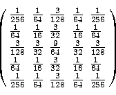
The above à trous algorithm has been discussed in terms of a single index, x, but is easily extendable to two-dimensional space. The use of the B₃ spline leads to a convolution with a mask of $5 \times 5$:

$$\left( \begin{array} {lllll} \frac{1}{256} & \frac{1}{64} & ... ...28} & \frac{1}{64} & \frac{1}{256} \end{array}\right) \nonumber$$

In one dimension, this mask is: $( \frac{1}{16}, \frac{1}{4}, \frac{3}{8}, \frac{1}{4}, \frac{1}{16} )$.

To facilitate computation, a simplification of this wavelet is to assume separability in the 2-dimensional case. In the case of the B₃ spline, this leads to a row by row convolution with $( \frac{1}{16}, \frac{1}{4}, \frac{3}{8}, \frac{1}{4}, \frac{1}{16} )$; followed by column by column convolution.

As for the one dimensional case, an exact reconstruction is obtained by adding all the scales and the final smoothed array:  

$$c_0(x,y) = c_{\rm p}(x,y) + \sum_{j=1}^{p} w_j(x,y).$$ (25)

Acknowledgements

We wish to thank Suzanne Madden for her kind help in the revision of the manuscript. We also would like to thank the anonymous referee whose comments had helped us to improve the quality of the paper.