3 The Atlas

Figure 1 shows spectra of A, G and M supergiants to provide identification for some of the strongest un-blended stellar absorption lines and the diffuse interstellar band at 8620 Å (which is sometimes the strongest feature in the spectra of O and B stars. The 8620 Å DIB will be investigated in detail later in this series). Apart from the Paschen and Ca II lines, the A-type spectra are dominated by strong N I absorptions, the G-type spectra present a large set of Fe I lines and the M-type show numerous and deep Ti I absorptions (cf. Table 4).

Figure 2 gives for the type G5 an example of what Figs. 5-28 (available only in electronic form) give for the other spectral types. They constitute the body of the present atlas. The spectra are arranged in luminosity sequences at selected spectral types. If available from the literature (cf. Table 2), the metallicity and the projected rotational velocity are given over each spectrum.

  

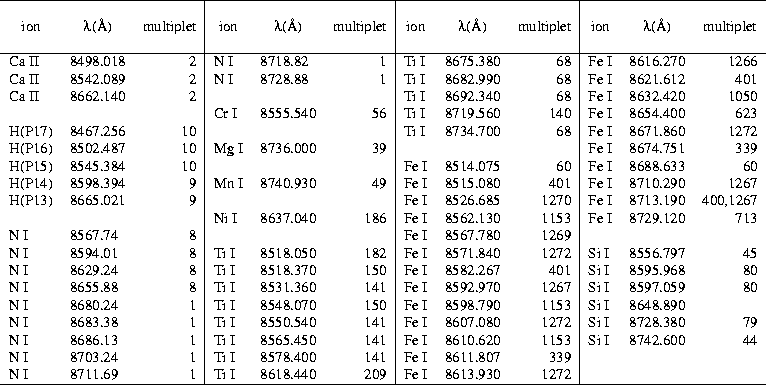
Figure 1: Sample spectra of supergiant stars with identification of some of the strongest un-blended absorption lines (cf. Table 5)

  

Figure 2: Luminosity sequence at G5. Metallicity and rotational velocities from the literature (cf. Table 2)

Figure 3 details how the selected wavelength region is the less affected by telluric absorptions in the near-IR (consecutive orders from an Echelle spectrum of a fast rotating B5 V star are plotted). Figure 4 (obtained from spectra of fast rotating main sequence B stars observed under high- and low-humidity conditions) shows in detail how marginal are the H₂0 telluric absorptions in the $\lambda\lambda$ 8500-8750 Å range. Such weak telluric absorptions are sometimes visible in the high S/N spectra of this atlas, particularly when stellar lines are broad and shallow like in hot and fast rotating stars (cf. Figs. 27 and 28).

 

Table 3: Our mapping of the MKK scheme in terms of spectral and luminosity classes (the "HD" preceding the star number is omitted)

 

Table 4: Identification of the major un-blended absortion lines over the $\lambda\lambda$ 8500-8750 Å range

 

Figure 3: Telluric absorptions in the near-IR from the spectrum of the fast rotating B5 V star HD 219688 ($V_{\rm rot}$sini = 340 km s-1). The stellar lines are the very broad and shallow absorptions (mainly hydrogen Paschen lines). The telluric lines are the much sharper lines. They are very abundant over the whole near-IR region, except for the arrowed portion of the spectrum which is the $\lambda\lambda$ 8500-8750 Å interval considered in this paper

 

Figure 4: Telluric absorption spectrum in the $\lambda\lambda$ 8500-8750 Å range obtained from spectra of some fast rotating B main sequence stars. The upper spectrum come from observations obtained with an average umidity of the air surroinding the telescope dome of 35%, the bottom one with an air umidity of 85%. The $\rm H_2O$ lines marked by dots are 8496.48, 8503.15, 8505.85, 8512.01, 8519.64, 8522.99, 8534.78 and 8540.82 Å

 

Figure 5: Luminosity sequence at M4

 

Figure 6: Luminosity sequence at M3

 

Figure 7: Luminosity sequence at M2. Metallicity and projected rotational velocity from literature (see Table 2)

 

Figure 8: Luminosity sequence at M1

 

Figure 9: Luminosity sequence at M0. Metallicity from literature (see Table 2)

 

Figure 10: Luminosity sequence at K7. Metallicity and projected rotational velocity from literature (see Table 2)

 

Figure 11: Luminosity sequence at K5. Metallicity and projected rotational velocity from literature (see Table 2)

 

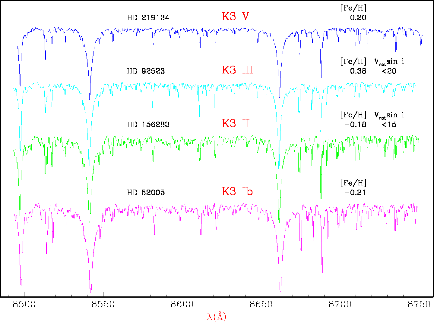
Figure 12: Luminosity sequence at K3. Metallicity and projected rotational velocity from literature (see Table 2)

 

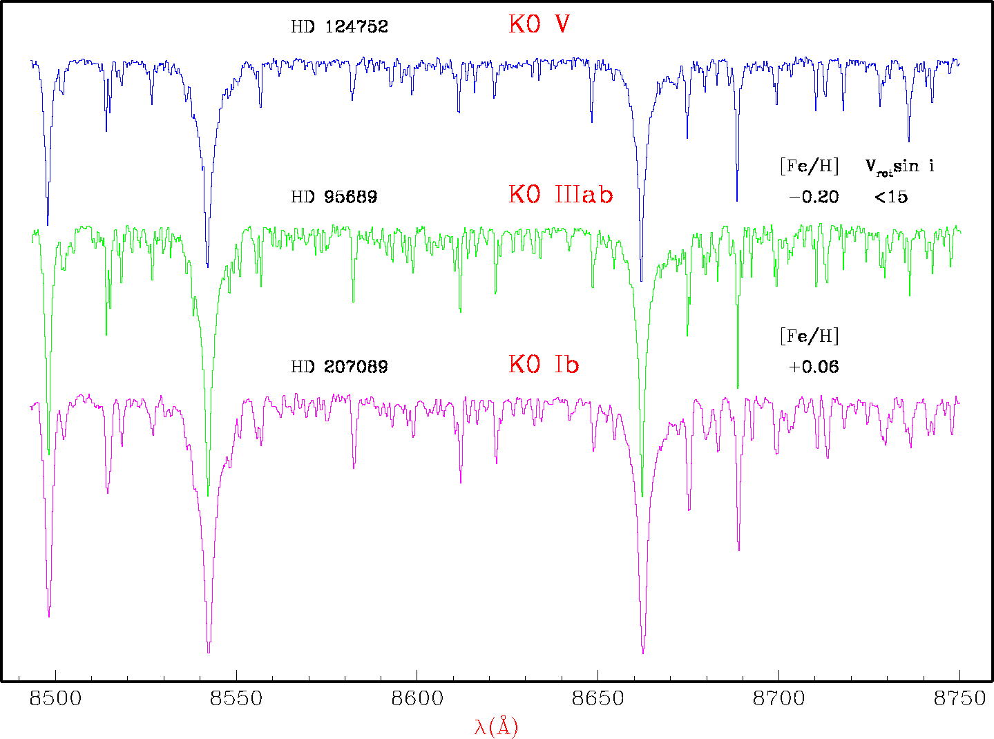
Figure 13: Luminosity sequence at K0. Metallicity and projected rotational velocity from literature (see Table 2)

 

Figure 14: Luminosity sequence at G8. Metallicity and projected rotational velocity from literature (see Table 2)

 

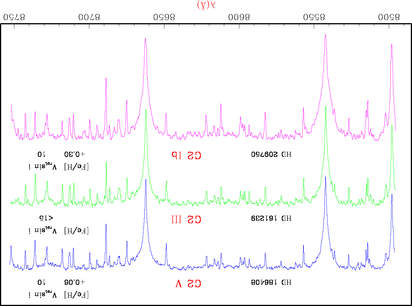
Figure 15: Luminosity sequence at G2. Metallicity and projected rotational velocity from literature (see Table 2)

 

Figure 16: Luminosity sequence at G0. Metallicity and projected rotational velocity from literature (see Table 2)

 

Figure 17: Luminosity sequence at F8. Metallicity and projected rotational velocity from literature (see Table 2)

 

Figure 18: Luminosity sequence at F5. Metallicity and projected rotational velocity from literature (see Table 2)

 

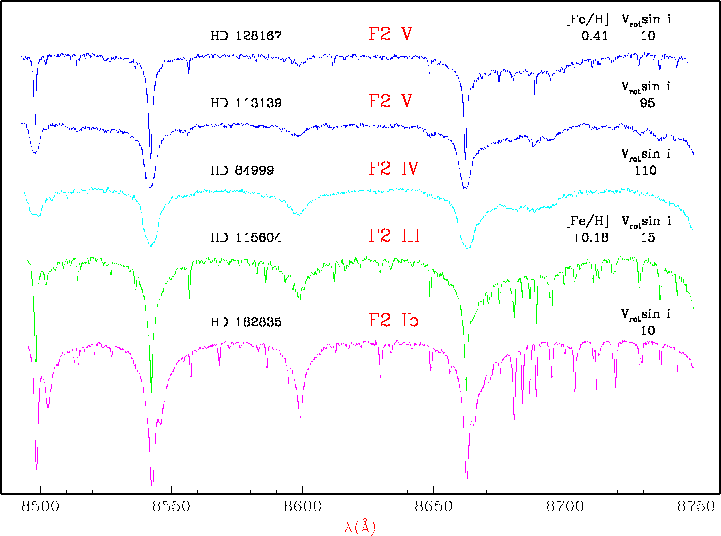
Figure 19: Luminosity sequence at F2. Metallicity and projected rotational velocity from literature (see Table 2)

 

Figure 20: Luminosity sequence at F0. Metallicity and projected rotational velocity from literature (see Table 2)

 

Figure 21: Luminosity sequence at A8-A9. Metallicity and projected rotational velocity from literature (see Table 2)

 

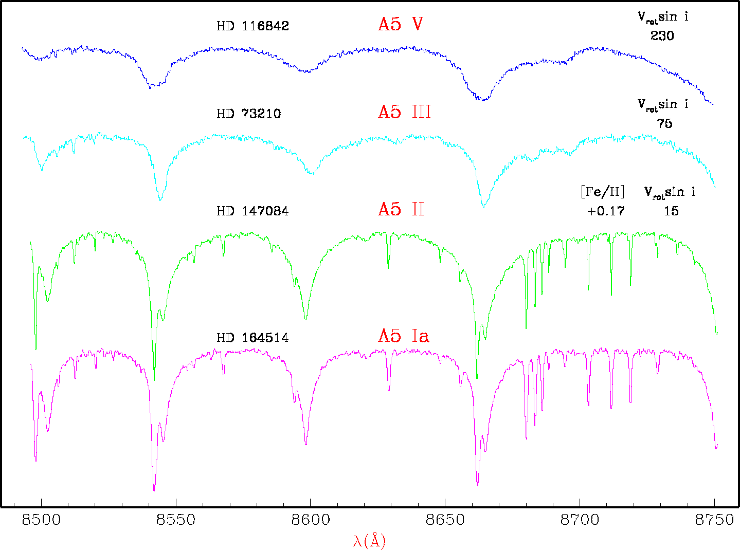
Figure 22: Luminosity sequence at A5. Metallicity and projected rotational velocity from literature (see Table 2)

 

Figure 23: Luminosity sequence at A3. Metallicity and projected rotational velocity from literature (see Table 2)

 

Figure 24: Luminosity sequence at A2. Metallicity and projected rotational velocity from literature (see Table 2)

 

Figure 25: Luminosity sequence at A0. Metallicity and projected rotational velocity from literature (see Table 2)

 

Figure 26: Luminosity sequence at B8. Metallicity and projected rotational velocity from literature (see Table 2)

 

Figure 27: Luminosity sequences at O9.5, B0, B3 and B5. Projected rotational velocity from literature (see Table 2)

 

Figure 28: Luminosity sequences at O6, O7, O8 and O9. Projected rotational velocity from literature (see Table 2)