4 Microvariability duty cycles

The observations presented in this paper can be used, along with the similar results obtained for northern objects by Jang & Miller (1995, 1997), to determine the microvariability duty cycles on the basis of a relatively large sample. Considering both sets of observations we have high-quality CCD variability data for 53 AGNs (23 southern and 30 northern objects). This sample is formed by 27 RQAGNs, 23 RL objects, and 3 XBLs. 74% of the radio-selected sources have displayed microvariations at the 99% confidence level within a single night. On the contrary, just 11% of the RQAGNs have shown variability under the same circumstances. This confirms that both AGN-types form distinct classes from the point of view of their microvariability (Miller & Noble 1996). In Fig. 9 we present an histogram where these results are summarized.

  

Figure 9: Histogram with variable (V) and nonvariable (NV) sources of each class (data from northern (Jang & Miller 1995, 1997) and southern (this paper) observations)

We can enlarge the RQ-sample by including the 13 objects monitored by Gopal-Krishna et al. (1993a,b, 1995) and Sagar et al. (1996) (we do not consider here the variable source 0838+359 because it is not a strict RQQSO). Taking into account the results of their observations the fraction of variable RQ objects is not significantly modified: 6 out of 40 (15%) sources present strong evidence of microvariability in their lightcurves (see Fig. 10).

  

Figure 10: Histogram for radio-quiet quasars taking into account different available data (see main text)

Several of the objects included in the Jang & Miller sample are not really QSOs, but rather Seyfert 1 (S1) galaxies. If we differentiate this group of lower luminosity sources from the rest of the sample we find that 7 out of 9 RLS1s (77.8%) displayed variability whereas just 2 out of 12 RQS1s (16.7%) showed similar behaviour.

Since some variable AGNs do not display variability all the time, duty cycles are best estimated not as the fraction of variable objects within a given class, but as the ratio of the time at which objects of the class are effectively varying to the total observing time for objects in that class. In this way we are taking into account the fact that there are nights in which usually variable AGNs do not present microfluctuations. Besides, since most sources have not been monitored during equals spans it is better to weight the contribution to the duty cycle by the hours each source was observed in each observing session. 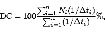Consequently, we define the following estimator for the duty cycle (DC) of objects of a given class:  

$${\rm DC}=100\frac{\sum^n_{i=1}N_i (1/\Delta t_i)}{\sum^n_{i=1} (1/\Delta t_i)}\%,$$ (2)

where $\Delta t_i=\Delta t_{i,{\rm obs}} (1+z)^{-1}$ is the duration (corrected by redshift) of a monitoring session of a source of the selected class, and N_i equals 0 or 1 if the object was NV or V during $\Delta t_i$, respectively.

Using this approach the duty cycles for RL, RQ, and XBL objects result of 68%, 6.9%, and 27.9%, respectively (see Fig. 11).

  

Figure 11: Microvariability duty cycles for X-ray selected BL Lac objetcs (XBLs), radio-quiet quasars (RQs) and radio-selected objects (RLs). The duty cycle is estimated according to Eq. (2)

The duty cycle of RQAGNs is, then, about one order of magnitude lower than the duty cycle of radio-selected AGNs. XBLs seem to present an intermediate level of activity, as previously noted by Heidt & Wagner (1998) from their intraday observations. We notice, however, that microvariability is not as frequent as optical intraday variability. The variability amplitudes for RBLs are also considerably smaller at timescales of a few hours: Heidt & Wagner (1996) estimate a mean IDV amplitude of $\sim\!28$% while for microvariations we obtain $<Y\gt~\sim 5$%.

In Table 5 we present the duty cycles estimated for the different types of objects (RQQSOs, RQS1s, RLQSOs, RLS1s, etc.). It is clear that these numbers must be considered with caution because of the limited size of the sample.

  

Table 5: Duty cycles for different types of AGNs from a sample of 53 objetcs

¹ "RLQSOs'' includes both radio-loud quasars and radio-selected BL Lacs.

Future observations could improve, and may be strongly modify, these estimates.

After the first version of this paper was completed we became aware of the comparative study of microvariability properties in RL and RQQSOs carried out by de Diego et al. (1998). On the basis of their analysis of the results of intranight observations of 17 radio-quiet and 17 radio-loud objects they claim, contrarily to what is suggested by all previous studies, that microvariability is a rather common phenomenon among RQQSOs, with duty cycles perhaps similar to those of RLQSOs. Their results, unfortunately, cannot be directly compared with those presented in this paper. Observational and analysis procedures are radically different between these two studies. de Diego et al. have observed each source between 3 and 9 times per night. Each observation consisted of five 1-min exposures of the target field. The resulting lightcurves have, consequently, lower temporal resolution than the ones discussed here. In addition, the microvariability analysis is made through the ANOVA procedure which determines observational errors directly from the object minus reference star observations within each set of data, and not from the scatter of comparison lightcurves as in our case. The problems of comparing results obtained from such different methods can be clearly appreciated considering the case of US 995, one of the most variable RQQSOs in de Diego et al. sample. After the first hour of observation, the brightness of this object increased about a tenth of magnitude, and dropped again when it was observed 1.5 hr later. The set of five 1-min exposures that contains the variation corresponds, according to de Diego et al., to a change of 0.17 mag in 120 s. Since the dispersion of the corresponding set of five points in a single comparison star is small, they conclude that the atmospheric conditions were good and that the feature in the lightcurve could be real. However, in the remaining 6 sets of observations of that night, the scatter of the comparison is similar to, or even considerably larger than, that displayed by the target. In abscence of other comparison lightcurves, there is no reason to claim that the QSOs was variable in a set of data and the comparison was not in the others. Moreover, an average comparison, as used in our research, would have provided almost certainly a larger scatter for the set of data in question, and the overall scatter of the QSOs lightcurve probably would not have satisfied a 2.6 $\sigma$ variability criterion. In order to produce a set of data that can be effectively compared with results obtained by other researchers, a larger number of comparison stars are required and the positions of these stars should be made explicit. This would allow to reproduce similar results with different instruments on the same objects, confirming the reality of the events.