2 Observations and data reduction

The objects included in our program are listed in Table 1, along with their 1950.0 coordinates, redshifts, apparent visual magnitudes, and classification of AGN-type.

  

Table 1: Observed AGNs

RBL: radio-selected BL Lac, XBL: X-ray selected BL Lac
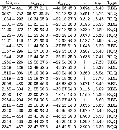RLQ: radio-loud quasar, RQQ: radio-quiet quasar.

They were selected from Véron-Cetty & Véron (1996), Drinkwater et al. (1997), and Padovani & Giommi (1995). All radio-quiet AGNs in our sample are QSOs with R<<1, where R is the ratio of radio (5 GHz) to optical (440 nm) flux densities. Radio-loud sources are highly polarized, flat-spectrum QSOs and BL Lac objects with R>1. We have distinguished in the BL Lac group two subgroups: radio-selected sources (RBLs) and X-ray-selected sources (XBLs). The radio-through-X-ray spectral energy distributions are different for these subgroups (Sambruna et al. 1996, Brinkmann et al. 1996) and there is strong evidence for the existence of very different duty cycles for them at intraday timescales (Heidt & Wagner 1996, 1998). These differences are probably reflecting different physical conditions in the relativistic jets of the objects (see, for instance, Sambruna et al. 1996).

Our observations were carried out during several observing runs in April, July, September, and December 1997, and April 1998 with the 2.15-m CASLEO telescope at San Juan, Argentina. This instrument was equipped with a liquid-nitrogen-cooled CCD camera, using a Tek-1024 chip with a read-out-noise of 9.6 electrons and a gain of 1.98 electrons/adu. A focal-reducer provided a scale of 0.813 arcsec per pixel, and the useful field of view was $\sim\!\!\!700$ pix in diameter, or roughly 9 arcmin on the sky. Field frames were then sufficiently large as to contain at least 6 non-variable stars of apparent magnitude similar to the AGN-target magnitude. These stars were used during the data reduction procedure for comparison and control purposes (see below).

Microvariability observations were performed entirely using a Johnson's V filter with integration times between 30 and 500 s depending on the source brightness and the observing conditions. The signal-to-noise ratio at the central pixel of the AGN was fixed at a level such that the count rate was about 25% below the saturation limit in each case. A number of calibration frames (bias and flat-field images) were taken each night before the beginning of the observations. The variability monitoring of each AGN lasted at least 3 hours in order to make our results directly comparable to those obtained by Jang & Miller (1995, 1997) for northern objects. As in their campaigns, several AGNs were observed during more than one night.

The data reduction was made following standard procedures with the IRAF software package running on a UNIX workstation. All object images were debiased and flat-fielded using the normalized dome flat images. Magnitude measurements of the AGNs were made relatively to non-variable field stars using the aperture photometry routine APPHOT. Differential lightcurves for each pair of objects in the frame were constructed and used for detecting variable stars or any anomalous behaviour (e.g. saturated stars). Two groups of well-behaved stars of similar magnitude to the target were determined for each AGN (usually three stars per group), and then an average magnitude was computed for each group in each frame. In Fig. 1 we show a finding chart for the first AGN listed in Table 1, where the object and the selected stars are marked.

  

Figure 1: CCD frame showing the field of 0537-441 (O) and stars used for comparison ($C_{1i},\;i=1,2,3$) and control ($C_{2i},\;i=1,2,3$). The image is 10 arcmin on each side; North is up and East to the left. Similar charts are available for all objects of the sample in the electronic version

In the electronic version of this article this figure contains similar frames for all objects of our sample in order to allow future researchers to make comparative studies using the same groups of stars. One of the averaged groups was used for comparison (<C_1i>) and the other for control (<C_2i>), in such a way that the differential lightcurve for each AGN (O) is presented as O-<C_1i>, while <C_1i>-<C_2i> provides a confident comparison curve. As in the Jang & Miller papers, the standard deviations ($\sigma$) of these latter curves are used as a measurement of the observational errors. The scatter $\sigma$supplies error estimates that are larger than the formal photometric errors and constitutes a more accurate determination of the actual errors along the entire variability monitoring of a given source. In most cases $\sigma$ is at the level 0.001-0.003 mag, and just in the worst cases occasionally reaches values of 0.01 mag.