

Up: Optimised polarimeter configurations for
Subsections
This paper originates from preparatory studies for the Planck satellite
mission. This Cosmic Microwave Background (CMB) mapping satellite is
designed to be able to measure the polarisation of the CMB in several frequency
channels with the sensitivity needed to extract the expected
cosmological signal.
Several authors (see for instance
Rees 1968;
Bond & Efstathiou 1987;
Melchiorri & Vittorio 1996;
Hu & White 1997;
Seljak & Zaldarriaga 1998),
have pointed out that measurements of the polarisation of the CMB
will help to discriminate between cosmological models and
to separate the foregrounds. In the theoretical analyses of the polarised power
spectra, it is in general assumed (explicitly or implicitly) that the errors
are uncorrelated between the three Stokes parameters I, Q
and U![[*]](/icons/foot_motif.gif) in the
reference frame used to build the polarised multipoles
(Zaldarriaga & Seljak 1997;
Ng & Liu 1997). However, the errors in the three Stokes
parameters will in general be correlated, even if the noise of the
three or more measuring polarimeters are not, unless the layout of the
polarimeters is adequately chosen. In this paper we construct
configurations of the relative orientations of the polarimeters,
hereafter called "Optimised Configurations'' (OC), such that, if the noise in all polarised
bolometers have the same variance and are not correlated, the
measurement errors in the
Stokes parameters I, Q and U are independent of the direction of
the focal plane and decorrelated. Moreover, the volume of the error
box is minimised. The properties of decorrelation and minimum
error are maintained when one combines redundant measurements of the same point of the
sky, even when the orientation of the focal plane is changed between
successive measurements. Finally, when combining unpolarised and data
from OC's, the resulting errors retain their optimised properties.
in the
reference frame used to build the polarised multipoles
(Zaldarriaga & Seljak 1997;
Ng & Liu 1997). However, the errors in the three Stokes
parameters will in general be correlated, even if the noise of the
three or more measuring polarimeters are not, unless the layout of the
polarimeters is adequately chosen. In this paper we construct
configurations of the relative orientations of the polarimeters,
hereafter called "Optimised Configurations'' (OC), such that, if the noise in all polarised
bolometers have the same variance and are not correlated, the
measurement errors in the
Stokes parameters I, Q and U are independent of the direction of
the focal plane and decorrelated. Moreover, the volume of the error
box is minimised. The properties of decorrelation and minimum
error are maintained when one combines redundant measurements of the same point of the
sky, even when the orientation of the focal plane is changed between
successive measurements. Finally, when combining unpolarised and data
from OC's, the resulting errors retain their optimised properties.
In general, the various polarimeters will not have the same levels of noise
and will be slightly cross-correlated. Assuming
that these imbalances and cross-correlations are small, we show that
for OC's the
resulting correlations between the errors on I, Q and U are also
small and easily calculated to first order. This remains
true when one combines several measurements of the same point of the
sky, the correlations get averaged but
do not cumulate.
Finally, we calculate the error matrix between E and B multipolar
amplitudes and show that it is also simpler in OC's.
In the reference frame where
the Stokes parameters I, Q, and U are defined, the
intensity detected by a polarimeter rotated by an angle  with respect
to the x axis is:
with respect
to the x axis is:
|  |
(1) |
Because polarimeters only measure intensities, angle can
be kept between 0 and  . To be able to separate the 3 Stokes
parameters, at least 3 polarised detectors are needed (or 1
unpolarised and 2 polarised), with angular
separations different from multiples of
. To be able to separate the 3 Stokes
parameters, at least 3 polarised detectors are needed (or 1
unpolarised and 2 polarised), with angular
separations different from multiples of  . If one uses
  polarimeters
with orientations
polarimeters
with orientations  for a given line of sight, the
Stokes parameters will be estimated by minimising the
for a given line of sight, the
Stokes parameters will be estimated by minimising the  :
:
|  |
(2) |
where  is the vector of measurements, and
  is their
  noise autocorrelation matrix. The
  matrix
| 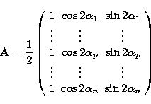 |
(3) |
relates the results of the n measurements to the vector of the Stokes parameters
 in a given reference
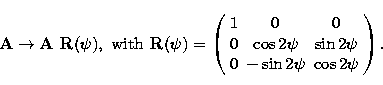
frame, for instance a reference frame fixed with respect to the focal instrument. If
one looks in the same direction of the sky, but with the instrument rotated by an angle
in a given reference
frame, for instance a reference frame fixed with respect to the focal instrument. If
one looks in the same direction of the sky, but with the instrument rotated by an angle
 in the focal plane, the matrix A
is simply transformed with a rotation matrix of angle
in the focal plane, the matrix A
is simply transformed with a rotation matrix of angle  :
:
|  |
(4) |
As is well known, the resulting estimation for the Stokes parameters
and their variance matrix  are:
and
are:
and
|  |
(5) |
Up: Optimised polarimeter configurations for
Copyright The European Southern Observatory (ESO)