According to GOES data, the flare started at 02:30 (all times are given in UT). The latitude of flare site was 25 $^{\circ }$ . The time interval of analysis is 00:23 - 06:00.

We must note that all estimates of height refer to the plane perpendicular to the line of sight. As the active region was already behind the limb, may be, all heights should be increased by $\leq 2.7\ 10^3$ km.

Time profiles of flux at frequencies 3.75, 5.7, 9.4, 17, and 35 GHz are plotted in semi-logarithmic scale in Figs. 1a and 2. The flux density measured with the 35 GHz polarimeter is affected by the atmospheric absorption, so the flux density may be overestimated after 05:00.

$\begin{figure} \epsfxsize 250pt \epsfbox{ds7864f1.eps}\end{figure}$

Figure 1: Microwave time profiles: a) total flux at different frequencies and maximum of brightness temperature at 17 GHz; b) effective height according to microwaves and Yohkoh/SXT data

The profile recorded at the SSRT (5.7 GHz) is not plotted around the peak of the burst since it is not reliable there due to multiple shifts of gain and presence of saturated records. Values of brightness temperature are available in NRH images. Peak brightness temperature was $1.2\ 10^9~$ K at 17 GHz.

We can distinguish three main stages of the flare according to the behaviour of the microwave burst (Table 1). Before the rapid increase, flux at 5.7 and 9.4 GHz exceeded flux at other frequencies, and the spectral peak $\nu _{\rm peak}$ was lower than 10 GHz. Then, in the interval near the burst maximum, $\nu _{\rm peak}$ was between 17 and 35 GHz. During the rapid decrease of the flux $\nu _{\rm peak}$ shifted again to a frequency of lower than 17 GHz. In the long-duration decay phase (after 03:22), the spectral index changed its sign again, and the relative value of flux increased with frequency. An exception - the interval during the sub-burst of 04:08 - 04:12 when the peak frequency was about 4 GHz.

**Table 1:** The stages of the flare
$\begin{tabular} {clcccl} \noalign{\smallskip} \hline \noalign{\smallskip} UT & C... ...$\simeq 4$\space & & gyrosynchrotron \\ \noalign{\smallskip} \hline\end{tabular}$

Variations of the height of microwave and soft X-ray sources above the limb are shown in Fig. 1b. Large height of the emitting region at 17 GHz before the flare is explained by the fact that this region was amorphous and extended up to significant heights without prominent brightness centres. When the flare started, two microwave sources became prominent: one close to the optical limb (17 GHz) and another one - at a height of about $10\ 10^3$ km (5.7 GHz). Later the relative brightness of the upper source increased, and this source began to be dominant at both frequencies.

Further, during more than two hours, a rising motion of the 17 GHz source was observed with the average velocity of about 3 km s^-1. Two intervals were outstanding: one during sharp rise of flux, when the velocity reached 15 km s^-1, and another one (03:16 - 03:22), during which the sources' height slightly decreased.

Variations of the height at 5.7 GHz during the first two stages were similar to that ones at 17 GHz. Near the peak of the burst, the low-frequency source was mainly higher. After that, the source at 5.7 GHz descended. In the decay phase, the weighted height of the sources at 5.7 GHz increased similarly to the height of 17 GHz ones, but it was about $15\ 10^3~$ km less.

The soft X-ray source was located lower than the microwave (17 GHz) one during the impulsive phase, and close to it in the decay phase after 03:22.

2.1.1 The first stage

Figure 2 shows expanded time profiles of total flux at different frequencies and the maximum of brightness temperature (T_B) at 17 GHz. It is remarkable that, on the average, the time profile of flux followed closely the exponential shape $\exp \left( \frac{t-t_0}\tau \right)$ during the first 17 minutes. For the flux $\tau \simeq 160$ s, so this interval exceeded $5\tau$ .

$\begin{figure} \epsfxsize 250pt \epsfbox{ds7864f2.eps}\end{figure}$

Figure 2: Extended time profiles of the total flux at different frequencies and the brightness temperature at 17 GHz in the initial stage

At 17 GHz, $\tau \simeq 200$ s for the maximum of T_B and the origin t₀ corresponds to 01:55. Note that before 01:50 the maximum of the brightness temperature within the flaring region decreased. It suggests that the real onset of the flare started at 01:55 indeed.

Growth rate of microwave emission after 02:48:53 went sharply up and both T_B and the flux increased in an order of magnitude within one minute at all the considered frequencies. The largest increase was observed at higher frequencies. After that, time profiles at 9.4 and 17 GHz became smoother.

Fine time structures were observed at all the frequencies on the background of the exponential growth. The shortest structures detected at 17 GHz in the records with 50 ms resolution were two similar prominent series of sub-second pulses around 02:44:50 and 02:45:10.

$\begin{figure} \epsfxsize 250pt \epsfbox{ds7864f3.eps}\end{figure}$

Figure 3: Fine temporal structure at different frequencies. Time resolution is 50 ms at 17 GHz, 56 ms at 5.7 GHz, 0.1 s at 9.4 GHz. The record of 9.4 GHz was averaged over 0.3 s

A series of sub-second pulses (spikes) observed at the end of this stage in SSRT 1-D scans since 02:53:45 to 02:54:45 was described by Altyntsev et al. (1995). The minimal duration of those spikes was less than the temporal resolution of the receiver (56 ms) and the maximal one was about 100 ms. Their flux ranged from 700 up to 1800 s.f.u. In this case, no corresponding pulses exceeding noise level were detected at the other frequencies.

$\begin{figure} \begin{center} \epsfxsize 400pt \epsfbox{ds7864f4.eps}\end{center}\end{figure}$

Figure 4: Structure of microwave sources in intensity and polarization observed at 17 GHz. Dashed lines - RCP, dotted - LCP. Three first sources are marked by digits in the upper row. Contour levels are (0.2, 0.5, 0.8) of the maximum of each polarity. The north is up

Let us consider relation between features in time profile and changes in spatial structure of the emitting region observed at 17 GHz (Fig. 4). Frames of the upper row correspond to the phase of exponential growth. It is remarkable that the structure of microwave sources varied considerably during the steady exponential growth of both T_B and flux.

In the frame of 02:37:00, the only compact positively-polarized (up to $38\%$ )source (1) was seen, and it was located close to the limb. Later the region of increased emission expanded along the limb to the north. Another positively-polarized source (2) appeared in the northern direction at 02:39:50 also close to the limb. Its polarization was up to $20\%$ . At 02:40:00, the third source (3) emerged above the second one at a height of $15\ 10^3~$ km (the frame of 02:43:50). This source had relatively low ( $\sim 5\%$ ) positive polarization (RCP).

Time profiles of brightness temperature for the three low-lying sources observed during the exponential growth are given in Fig. 5. The bottom of the figure is the result of subtraction of the exponential trends from each of the curves. We can see that the time profiles of the sources 2 and 3 are very close, and the profile of the source 1 differs significantly from them. The sources 2 and 3 were located radially with a distance between them of $14 \ 10^3$ km. From the bottom of this figure we can see similar oscillations of the brightness temperature with a period of 70 s occurred in these sources. There is a delay of peaks in the source 3 with respect to the source 2 by $\simeq 6.6$ s. If these sources corresponded to the same loop, then the delay may be due to difference of trapping time in these sources. It also can be explained by motion of some exciting agent from below with a velocity of $\geq 2\ 10^3$ km s^-1. Another geometry was also possible. The sources 2 and 3 may correspond to different loops intercrossing and interacting behind the limb.

The increase of flux in the interval 02:44:00 - 02:44:30 was connected with appearance of a new positively polarized source at the same height as the source 3 towards south-east (Fig. 4, the upper right frame). The brightness centre in I-images moved in the southern direction, to a position between the regions of opposite polarization. Note, that both sets of sub-second pulses occurred at 17 GHz were located in this brightness centre ( $15\ 10^3$ km above the limb). Sizes of their sources were close to the beam size of NRH (7 thousand km $\times 10$ thousand km).

The sharp increase of T_B and flux at the end of the first stage corresponds to a fast extension of an RCP source pressed to the negatively polarized region from below (02:49:50). Starting from this time, the source in I-image became dome-like with the lower edge located $\simeq 15\ 10^3~$ km above the optical limb. This emitting region rapidly expanded to the south-west direction and then varied negligibly till 03:20. The peaks at 02:53:55 and 02:58:50 were associated with reconstruction of the LCP-source and enlargement of the nearest part of the RCP-source (see Fig. 4, 02:53:50). The degree ofpolarization did not exceed $20\%$ for these sources.

$\begin{figure} \epsfxsize 250pt \epsfbox{ds7864f5.eps}\end{figure}$

Figure 5: a) Oscillatory initial part of the time profiles of brightness temperature in three low-lying sources; b) expanded time profiles of the sources 2 and 3 with subtracted exponential trend. The time interval of the lower plot is marked in the upper one by vertical lines

To compare structures visible in 2-D images at 17 GHz and 1-D scans at 5.7 GHz, let us consider the Figs. 1b and 6. During the first stage of the flare, the height of the sources above the limb increased at both 17 and 5.7 GHz. The sources were close till the sharp rise of flux (Fig. 6, 02:45:00). A short-duration increase of the height prominent at 5.7 GHz and faint at 17 GHz occurred at 02:54. The brightness centre at 5.7 GHz became $10\ 10^3~$ km higher than the 17 GHz source at this time. It indicates appearance of a new source which contributed considerably to the total flux at 5.7 GHz, but was not seen at 17 GHz. Note that the source of 5.7 GHz sub-second spikes coincided with the brightest point of the background burst at this frequency, i.e. with the source located above the region emitting at 17 GHz.

$\begin{figure} \epsfxsize 250pt \epsfbox{ds7864f6.eps}\end{figure}$

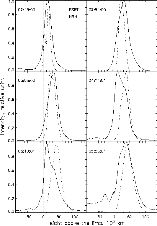Figure 6: A set of 1-dimensional scans obtained at the SSRT and computed from images obtained at the NRH during the flare

2.1.2 The second stage

$\begin{figure} \epsfxsize 250pt \epsfbox{ds7864f7.eps}\end{figure}$

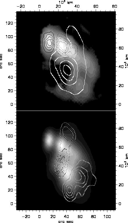Figure 7: The loop appeared during the sub-burst at 04:10 UT: a) colour - difference of I-images of 04:10 and 04:08, black contours - difference of V-images of 04:10 and 04:08, white contours - I-image of 04:06. b) colour - I-image of 04:10, contours - V-image of 04:06. Broken lines - negative polarization. To reveal the whole shape of the loop visible in the subtracted I-image, non-linear display was applied. Contour levels of polarization are (0.2, 0.4, 0.6, 0.8) of the maximum of each polarity ( $-10\%$ and $+25\%$ ). Contour levels of I-image of 04:06 are $(0.5, 1.5, 2.5, 3.5)\, 10^6$ K

Increasing of the flux continued at lower frequencies. At 5.7 GHz, this increase was due to appearance once more of the higher source invisible at 17 GHz (Figs. 1b and 6). Its height was close to that one at 02:54. This source disappeared near 03:10 when the decay at 17 GHz was accelerated.

After 03:00, Yohkoh data is available. At 03:00, a compact hard X-ray source was observed whose height $34\ 10^3$ km (Nakajima et al. 1998) was close to the height of the upper source at 5.7 GHz. The soft X-ray source was significantly lower than the microwave sources at both frequencies and the HXT one at this time. The height of the soft X-ray source above the limb was increasing, and in the end of the second stage, the heights of the microwave sources and the soft X-ray kernel became close.

2.1.3 The third stage

It lasted until the end of the observations. The behaviour of the burst at 17 and 35 GHz was characterised by large time scales of variations (except for rather faint sub-bursts). Note also that the time profiles at lower frequencies were not smooth: a series of sub-bursts during two hours is detectable in semi-logarithmic profiles at 3.75 and 5.7 GHz. Corresponding enhancement was observed at 17 and 35 GHz only for the most powerful sub-burst (04:12). Microwave emission of at least two components was obviously present within the interval 04:08 - 05:40, i.e. slow decay of high-frequency residual emission of the upper source, and weaker low-frequency sub-burst emission of the lower sources.

The upper source at 17 GHz shifted above the LCP-region and moved upwards extending to the north (Fig. 4, the bottom row). Polarization was small, but, as before, the marked brightness centre in I-images was situated between the regions of opposite polarization. The brightness centres in soft X-rays and in 17 GHz image became close in this stage. The lower source can be seen in 17 GHz map during the relatively short interval near 04:10 (Fig. 4). In Fig. 7a, the difference of two images obtained at 04:10 and 04:08 is shown. We investigated time profiles of T_B in different points of the image. No direct relation between the lower impulsive and the upper quasi-stationary sources was found: the impulsive increase of the brightness temperature in the lower source had no response in the upper one, although it marked a loop enveloping the upper source. The impulsive brightening in the enveloping loop was delayed with respect to the lower source. It may be interpreted as trapping of the electrons in the upper part of the loop with $\sim\! 100$ s.

The behaviour of the effective source's height at 5.7 GHz (Fig. 1b) is due to variations of relative brightness of two sources separated in height. They can be distinguished in SSRT 1-D scans in the interval 04:12:51 - 05:54:49 (Fig. 6). The lower source had a height of $\simeq\! 10\ 10^3$ km and the upper one moved upward together with the 17 GHz source. The degree of polarization at 04:10 was $29\%$ for the lower RCP-source, and $13\%$ for the LCP-region.

2.1.4 Summary of the development of the spatial structure

A region of enhanced microwave emission was observed a few hours before the flare high in the corona, where the flaring sources appeared later. Extended weakly polarized regions existed on the periphery of this wide area. The positive ones were lower, close to the optical limb. In the first three pictures (Fig. 8), two oppositely-polarized regions moved towards each other. This motion indicates movement of components of the magnetic structure, and also suggests a shear motion at footpoints of magnetic loops. The structure of the polarized region in the last picture became similar to that observed at the beginning of the flare. The degree of polarization did not exceed 10%.

Generalised pictures of the flare development are shown in Fig. 9. These pictures were obtained by addition of all the frames, each of which was previously normalised to unit.

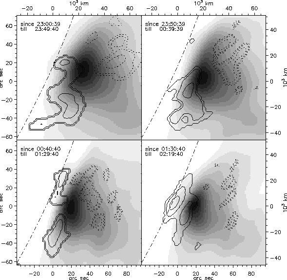$\begin{figure} \begin{center} \epsfxsize 420pt \epsfbox{ds7864f8.eps}\end{center}\end{figure}$

Figure 8: The structure of microwave sources in intensity (I; colour) and polarization (V; contours, dotted are negative) before the flare. Each frame was averaged over 49 minutes. Contour levels are (0.2, 0.5, 0.8) of the maximum of each polarity

Low-lying sources with high degree of polarization were observed in the beginning of the flare. During the first stage, sources in I-images (Fig. 9a) moving towards north-west got the dome-like shape and then enlarged towards south-west. In the second stage, when the intensity decreased, the shape and the size of the microwave source were not changed considerably. In the third (last) stage, the source in I-images expanded slowly and moved towards north-west. Note that sometimes in this stage also a source located close to the optical limb was observed.

More complicated structure is seen in the V-map averaged during the flare (Fig. 9b). RCP-sources appeared one by one around the LCP-sources. This large-scale structure as a whole did not change itself significantly during the flare, and its parts came subsequently in sight.

Consequently, the main structural components of the area emitted in microwaves before and during the flare were large-scale systems of intercrossed magnetic ropes. Cross sections of, at least, three of them were seen in polarization structure. The first system was represented by the low-lying strongly polarized RCP sources which corresponded to the top parts of low loops. The other two large-scale systems were represented by the regions of weak opposite polarization which were seen high in the corona in the main impulsive phase (in the late first and second stage) and in the third stage. In general, the situation can be characterised as a multi-level and a multi-loop one both at the onset and in the end of the flare.

$\begin{figure} \begin{center} \epsfxsize 200pt \epsfbox{ds7864f9.eps}\end{center}\end{figure}$

Figure 9: The maps averaged over the whole sets of 17 GHz maps in intensity (I; a) and polarization (V; b) obtained during the flare are shown by colour. Half-height contours of the sources in I- and V-images are shown for some instants. Three different stages of the burst are marked by different line styles: solid - the $1^{\rm st}$ stage, dotted - the $2^{\rm nd}$ stage, dashed - the $3^{\rm rd}$ stage

2 Observations

2.1 Development of the burst

2.1.1 The first stage

2.1.2 The second stage

2.1.3 The third stage

2.1.4 Summary of the development of the spatial structure