2 The mini-survey

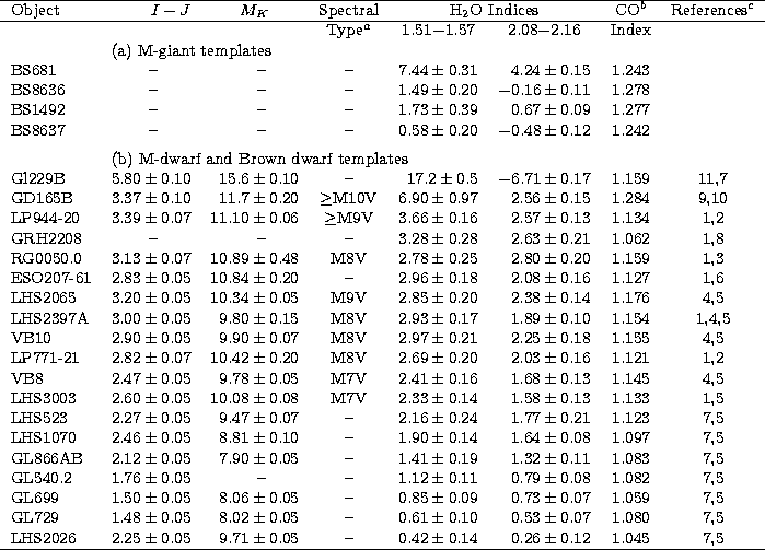
We have carried out a "Mini-survey'' with spectroscopic follow up on the very low-mass star and brown dwarf candidates contained in $\approx$1% of the DENIS survey data. The "Mini-survey'' data are representative of the survey quality, and its results can therefore be scaled to evaluate the brown dwarf content of DENIS. The image data from the high latitude part ($\vert b_{\rm II}\vert\gt 20-30$$^\circ$) of 47 survey strips (for a total surface area of 230 square degree), as produced by the Paris DAC, were hand processed to create catalogs of I, J and K$^\prime$ photometry. From these we identified a sample of objects for which infrared H- and K-band spectroscopy was carried out, in order to "clean'' the dirty sample and evaluate its level of contamination.

  

Table 1: Mini-survey strips with 50% completeness limits

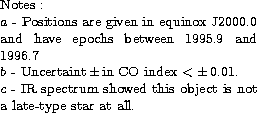
Notes: a - Strips centered on: -13$^\circ$ span $\delta=+2$$^\circ$ to -28$^\circ$;-43$^\circ$ span $\delta=-28$$^\circ$ to -58$^\circ$; -73$^\circ$ span $\delta=-58$$^\circ$ to -88$^\circ$.

2.1 The DENIS data

DENIS observations are carried out on the ESO 1m telescope at Cerro La Silla (Chile), with a purpose-built three channel infrared camera (Copet et al. 1998). Dichroic beam splitters separate the three channels, and focal reducing optics provide a 12$^\prime$ field of view for all the channels. The detectors used give image scales of 3$^{\prime\prime}$/pixel on the $256\times 256$ NICMOS3 arrays used for the two infrared channels and 1$^{\prime\prime}$/pixel on the $1024 \times 1024$ Tektronix CCD detector of the I channel. A focal plane micro-scanning mirror is used to obtain 1'' sampling for the two infrared channels. Cold filters define the spectral band-passes which are close to Gunn i, $J_{\rm{CIT}}$, and Mauna Kea $K_{\rm short}$ (Copet et al. 1998). The sky is scanned in a step and stare mode, along 30 degrees strips at constant right ascension. These strips are centered at $\delta = -13\hbox{$^\circ$},\, -43\hbox{$^\circ$}\ \& -73\hbox{$^\circ$}$, and are the basic DENIS observing unit. Photometric standards are observed at the beginning and end of each strip. Strip spacing and image spacing within a strip are both 10', providing 20% overlap in right ascension. Integration time is $\sim 10\,$s.

The 47 strips used for the Mini-survey (see Table 1) were chosen to maximise galactic latitude and to obtain useful right ascension coverage during our follow-up spectroscopic observing runs - the table is split into two sections as slightly different selection criteria were used for the northern and southern Galactic hemisphere samples. The image data were obtained from the Paris DAC and had been processed with version 4.2 of the standard pipeline software (Borsenberger 1997). The background levels are derived from a local clipped mean along the strip. Flat-field corrections are derived using observations of the dawn sky.

When this project was commenced the Leiden source extraction pipeline was not yet operational. Source detection and photometry was therefore performed in Grenoble, using the SExtractor package (Bertin & Arnouts 1996). Sources were detected after smoothing the image with a 2$^{\prime\prime}$ FWHP kernel, requesting a minimum of 5 contiguous pixels above a threshold of 1.5 standard deviations of the original image for the southern sample and 2.5 for the northern one. Adaptive aperture photometry was then extracted from the original unsmoothed image. The images of the closest photometric standards were identically processed, and used to define the zero point of the instrumental magnitudes. Since the objects of interest in our survey are close to our limiting magnitude, their photometric uncertainties are significant. As a result, we have not attempted to apply the small corrections appropriate to the airmass difference between our standard and strip observations, nor did we correct for colour terms.

Completeness curves were estimated for each strip by fitting low order polynomials (n = 1-3) to the brighter part of the differential number count (i.e. Log(N)/Log(S)) curve for that strip, and using this fit to normalise the Log(N)/Log(S) curve. This normalised Log(N)/Log(S) curve was then used to evaluate the magnitude at which the strip is 50% incomplete. A typical example is shown in Fig. 1 and the resulting completeness limits for each strip are listed in Table 1. The variation in completeness level reflects changes in the sky level - due to the moon phase for I, and to ambient temperature variations for K.

  

Figure 1: Completeness plot for Strip 3128

 

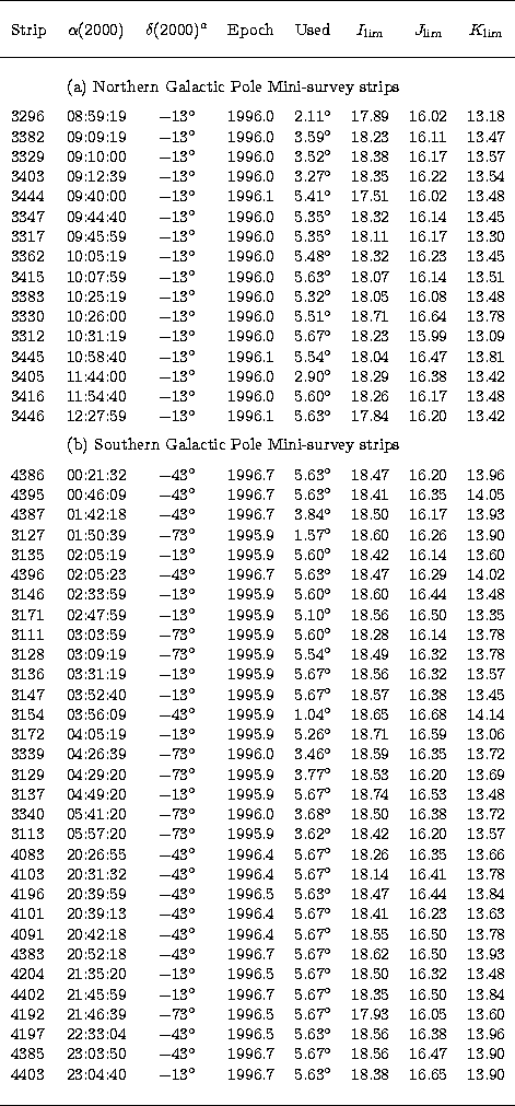
Figure 2: I band finding charts for the objects listed in Table 2. The size of this chart is ${\sim}\,3.5'\times3.5'$. North is up and East is left

 

Figure 3: I band finding charts for the objects listed in Table 2. The size of this chart is ${\sim}~3.5'\times 3.5'$. North is up and East is left

 

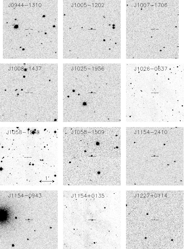Figure 4: I band finding charts for the objects listed in Table 2. The size of this chart is ${\sim}~3.5'\times 3.5'$. North is up and East is left

 

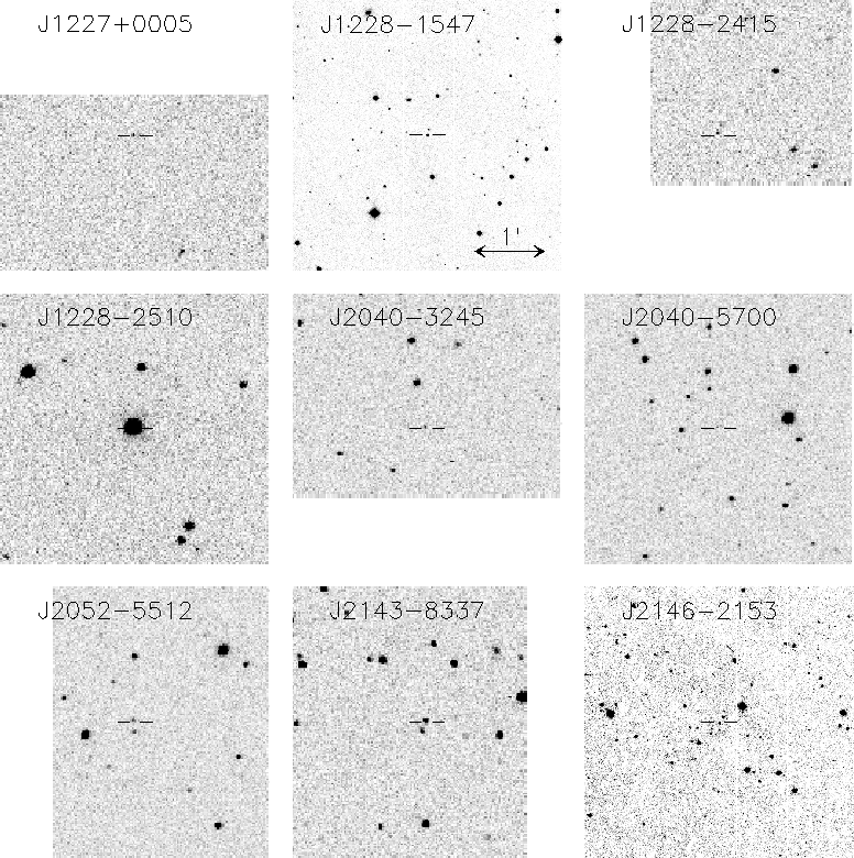Figure 5: I band finding charts for the objects listed in able 2. The size of this chart is ${\sim}~3.5'\times 3.5'$. North is up and East is left

2.2 Spectroscopic sample selection

Even though VLMs and brown dwarfs are brightest at near-infrared wavelengths, they are still vastly outnumbered in our flux limited samples by intrinsically brighter and more distant stars. As an illustration, the present mini-survey has obtained photometry at I and J for some $6\ 10^5$ stellar objects, of which less than 50 were finally retained as VLM/BD candidates. With such a low selection fraction it is essential that the selection scheme has a very low false alarm rate, since even a small "blue leak'' of 0.01% would still produce a sample dominated by G and K dwarfs.

Contamination by distant disk red giants increases at low galactic latitudes, as does the general stellar background within which we have to search for the brown dwarf signal. We initially imposed a galactic latitude limit of $\vert b_{\rm II}\vert \gt 30$$^\circ$ - though this was later relaxed to $\vert b_{\rm II}\vert \gt 20$$^\circ$ as our confidence in the processing increased. All objects in 650$^\prime$$\,\times 550$$^\prime$ and 280$^\prime$$\, \times 160$$^\prime$ zones centered on the LMC (5$^{\rm h}$23.6$^{\rm m}$- 69$^\circ$45$^\prime$) and the SMC (0$^{\rm h}$52.7$^{\rm m}$ - 72$^\circ$50$^\prime$) were also rejected, to avoid contamination by cool Magellanic Cloud giants.

Objects detected within 20$^{\prime\prime}$ of the edge of an image were ignored, as were objects with clearly non stellar parameters. At the relatively bright fluxes sampled by DENIS, galaxies are rare and typically much bluer than late M dwarfs, and would therefore have been eliminated by colour alone. Morphological rejection was primarily implemented to exclude cosmic rays and some optical ghosts. Finally, all sources within a $6\times 6$ pixel zone 86pixels north of every bright (J<10, K<8) source were ignored. Multiple reflections within the DENIS dichroic splitters produce a faint infrared ghost, which has no counterpart at I and can thus have extremely red apparent colours.

The three individual channels were then merged, using the I channel as a position reference. A linear transformation (offset, rotation, and scaling factor) between the other channels and this master channel was determined by minimizing the sum of the squared distances between all unsaturated stars brighter than I<17, J<15 and K<13.4. The J and K object lists were then searched for matching objects within 3$^{\prime\prime}$ of each I object to produce a three colour catalog for each strip. Because source confusion is never a problem at the galactic latitudes analysed here, this simple procedure was extremely effective.

Candidates were then selected in the three colour catalogs. To avoid contamination by cosmic rays, sources were required to be detected in at least two pass bands. For the objects of interest, J is always the most sensitive passband, so two classes of objects were selected: (1) objects with a very red I-J; and (2) objects with J and K detections but no I detection. The latter criterion aimed to select extremely low temperature objects ($T_{\rm eff} \approx 1000$ K) with colours similar to Gl229B - visual inspection of all these candidates revealed no reliable detections beyond objects also selected on I-J. In the remainder of this paper we consider only objects with very red I-J colours. The northern sub-sample was processed first, and we selected all objects with I-J> 2.75, or I-J> 2.2 for the brighter ones. In view of the large number of selected objects with large photometric errorbars (and presumably with an actual I-J bluer than 2.5), we changed the selection criteria for the southern sample and retained all objects with $(I-J)-\sigma(I-J)\gt 2.5$.

Inspection of the image data for these selected objects showed that $\sim$80% were contaminated by bad pixels or cosmic rays, and had much bluer intrinsic colours. This large artefact fraction illustrates a well known difficulty when looking for needles in haystacks (the population of interest represents less than 0.01% of the number of detected stars). It suffices that a very small fraction of the 99.99% of higher mass stars is affected by a bad pixel or a cosmic rays for it to dominate the very low mass star and brown dwarfs region of the color-color diagram. Since such contamination could not be selected against using the extracted source parameters, we visually inspected the image data for all the initially selected VLM/BD candidates. One reason for this relatively high level of sample contamination is that version 4.2 of the Paris DAC software used incorrect bad pixel flagging - future DENIS data will be significantly improved in this respect. Cosmic rays will also be identified with increased precision in future DENIS data by a neural network classifier, to be used in the next generation of the Leiden DAC extraction software (E. Bertin, private communication).

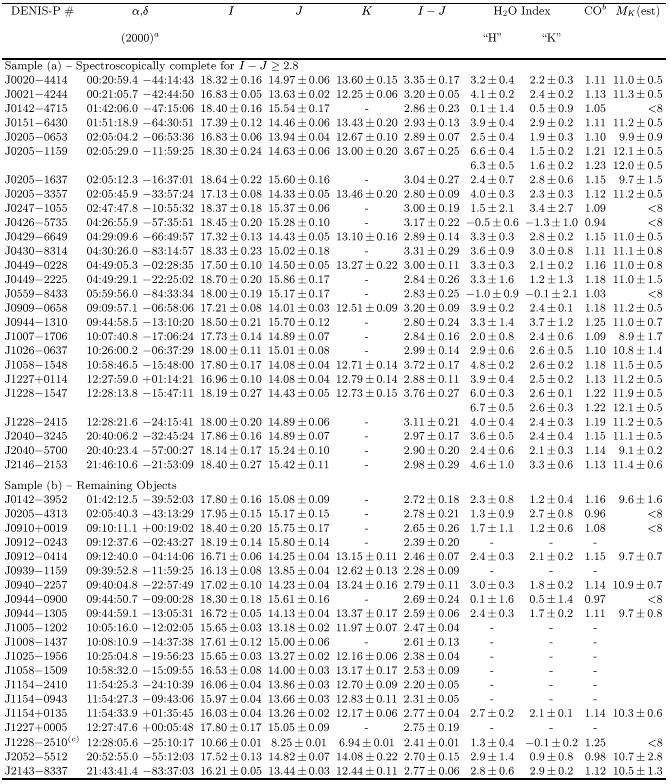
The objects remaining after this visual sample culling are listed in Table 2. Table 2a shows the list of objects identified for spectroscopic follow-up which constitute a sample with I-J> 2.8. Table 2b lists the remaining objects selected from the DENIS data. The positions provided are based on the telescope encoder readings, and are accurate to $\pm \,10-20$$^{\prime\prime}$,Much better position will be produced by the final DENIS pipeline.

  

Figure 6: I-J/J-K colour-colour diagram for the objects selected from the DENIS strips and for templates from the literature. Open triangle: spectroscopically observed; filled triangle: not spectroscopically observed; solid circle: template M dwarfs from Leggett (1992) and Tinney, Mould & Reid (1993). All DENIS objects redder than our completeness limit of I-J=2.8 were spectroscopically observed

The listed photometric errors are internal errors determined by the photometry package, and will thus be underestimates for the brighter stars. Figure 6 presents the selected objects detected in all three colours in a colour-colour diagram, I-J versus J-K.

  

Table 2: The DENIS Mini-survey Spectroscopic sample

2.3 Infrared spectroscopy

Infrared spectroscopic observations were carried out on the 3.9 m Anglo-Australian Telescope (AAT) on the nights of 1996 April 9 and 10 (UT) and 1996 October 21 and 22 (UT). On both runs the Infra-Red Imaging Spectrograph (IRIS - Allen et al. 1993) was used in its cross-dispersed HK echelle mode. This provides complete wavelength coverage from $1.438 - 2.536\,\mu$m, at a resolution of $\lambda/{\Delta\lambda} = 440$, and a dispersion of $\lambda/{\Delta\lambda} = 780$. A slit of width 1.4$^{\prime\prime}$ and length 13$^{\prime\prime}$ was used.

Observations were typically of 20 minutes total integration time, and were made with the object being nodded between two positions on the slit. Reductions were performed using the Figaro data reduction package (Shortridge 1993) and followed a standard procedure: the data were sky subtracted using pairs of nodded observations, straightened to remove the curvature of the echelle orders and the wavelength dependent "tilt'' of the IRIS slit, and extracted using a modified version of the Figaro ANAL routine to remove any residual sky spectrum left after pair-subtraction. A variety of arcs (Ne, Ar, Cu, Hg and Xe) were used to construct a wavelength calibration good to $\pm \,2.5$ Å, which was applied to all the spectra.

Spectra of late F-type and early G-type stars were used to create flux calibrations. Because of the water vapour content at the AAT site, we did not attempt to correct for absorption near the atmospheric H₂O bands. Standards were observed every few hours, at airmasses within $\pm\, 0.2$ of the program object observations. The observed standards had their H Brackett lines corrected by hand. The lines were identified by dividing each standard by a G-type spectrum in which the H lines are negligibly weak. The CO bands beyond 2.2 $\mu$m were not corrected, as these were weak (i.e. less than a few percent) in even the latest G5 standards. Lastly, the photometry of Carter & Meadows (1995) was used to put these standards on an approximate flux scale. While the relative fluxes obtained for our program stars are good to better than 5%, the absolute fluxes are no better than $\pm \,30\%$.

  

Figure 7: IRIS HK echelle spectra for representative DENIS dwarfs from Table 2. All spectra have been normalized by their flux integrated between 2.09 and 2.11$\mu$m, and offset by steps of 0.5 from the preceeding object. Objects are shown ordered by the estimated MK derived as described in the text. The dashed lines show the wavelength ranges where terrestrial H2O absorption make the spectra unreliable. The dotted boxes show the wavelength ranges over which the H2O indices described in Sect. 2.4.2 were measured

  

Figure 8: IRIS HK echelle spectra (continued). See Fig. 7 caption

  

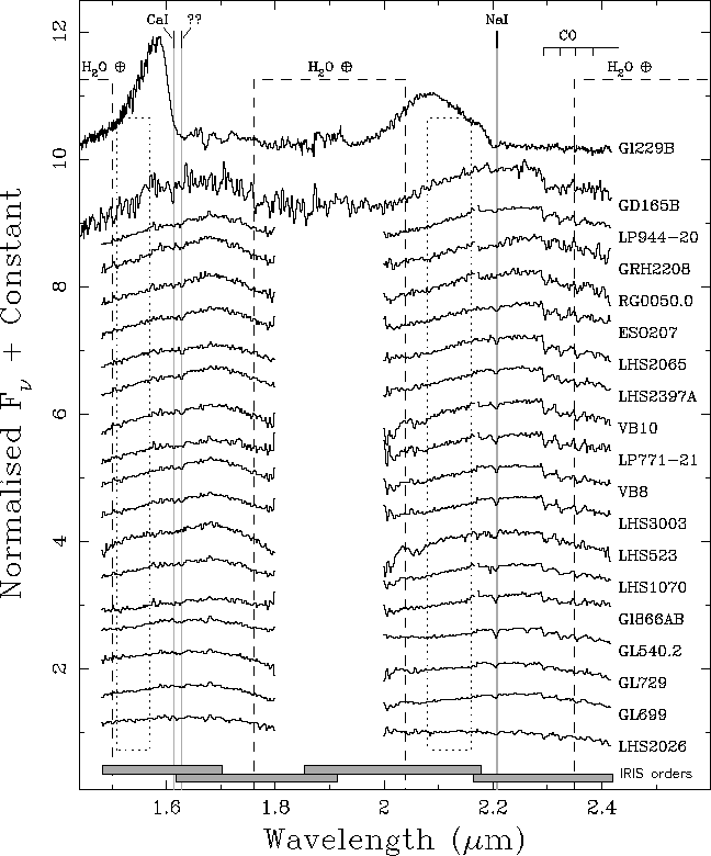Figure 9: IRIS HK echelle spectra of the template dwarf objects listed in Table 3. All spectra have been normalized by their flux integrated between 2.09 and 2.11$\mu$m, and offset by steps of 0.5 from the preceeding object, with the exception of of Gl229B which has been offset by 1.5. The dashed lines show the wavelength ranges where terrestrial H2O absorption make the spectra unreliable. The dotted boxes show the wavelength ranges over which the H2O indices described in Sect. 2.4.2 were measured

  

Table 3: Template object spectral classifiers

Notes:
a - Spectral types are due to Kirkpatrick et al. (1997b) and Kirkpatrick et al. (1995),
b - uncertainty in CO ratio $< \pm 0.005$.
c - References for photometry and astrometry: (1) Tinney 1996; (2) Kirkpatrick et al. 1997b; (3) Reid & Gilmore 1981; (4) Monet et al. 1992; (5) Leggett 1992; (6) Ruiz et al. 1991; (7) Gliese & Jahreiss 1991; Gliese 1969; (8) Gilmore et al. 1985; (9) C.Dahn, private communication, see Sect. 3.2; (10) Tinney et al. 1993; (12) Matthews et al. 1996.

  

Figure 10: IRIS HK echelle spectra of the template giants (cf. Table 3), and the two DENIS objects classified as giants in Sect. 2.4.1. All spectra have been normalized by their flux integrated between 2.09 and 2.11$\mu$m, and offset by steps of 1.0 from the preceeding object, with an added step of 1.0 between the template and target stars. The dashed lines show the wavelength ranges where terrestrial H2O absorption make the spectra unreliable. The dotted boxes show the wavelength ranges over which the H2 indices described in Sect. 2.4.2 were measured

Figures 7 and 8 present a sample of the spectra obtained for the program objects listed in Table 2. A sample of comparison objects was also observed - in particular four late-type giants, and a large number of late-type dwarfs. These are listed in Table 3 and shown in Figs. 9 and 10. Because the AAT is a relatively low-altitude site, it is not possible to make observations through the atmospheric water vapour bands. These have been marked on the figures. However, even outside these regions both the dwarf and giant spectra show the broad stellar H₂O absorption bands characteristic of these low temperature atmospheres. CO bandheads are seen from $2.3-2.4\,\mu$m in all the spectra, though some of the giant spectra also show CO in the $1.6-1.7\,\mu$m region. Numerous spectral lines due to neutral metals are also seen - in particular, Na I $\lambda\,2.20\,\mu$m and Ca I $\lambda\,1.614\,\mu$m (Tinney et al. 1993). There is also a strong absorption in many of the dwarfs at $\lambda\,1.627\,\mu$m, which remains unidentified.

2.4 Infrared spectral classification

2.4.1 Giant/dwarf discrimination

A comparison of the giants and dwarfs in Figs. 9 and 10 shows that for high signal-to-noise ratio observations the presence of Na in absorption at 2.20 $\mu$m indicates that the atmosphere is at high (i.e. dwarf) gravities (Jones et al. 1994; Tinney et al. 1993). However, for much of our data, such a criteria cannot be used because of the signal-to-noise available. 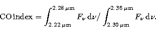A giant dwarf discriminant which can be used at lower S/N is the strength of CO bandhead at 2.29 $\mu$m. Following Jones et al. (1993) we therefore define a CO index as the ratio of the integrated flux in bands at $(2.22-2.28)\,\mu$m and $(2.30-2.36)\,\mu$m.

$${\rm CO}\, {\rm index} = \int^{2.28\,\mu{\rm m}}_{2.22\,\mu{... .../ \int^{2.36\,\mu{\rm m}}_{2.30\,\mu{\rm m}} F_\nu\,{\rm d}\nu.$$ (1)

Figure 11a shows this CO index as a function of I-J colour, for the comparison objects we observed. No I-J colours are available for the giants in our comparison sample, and as these objects are all long-period variables, colour information would not necessarily be meaningful. The measured giant ratios are thus shown as arrows at the appropriate CO index level. The expected dependence is seen, in that CO is much stronger in giants than in dwarfs. We therefore define a criterion that if the CO index > 1.24 the object is classified as a giant. This classifies two sources, as giants - DENIS-PJ1228-2510 and J0944-1310.

The giant classification of DENIS-PJ1228-2510 is supported by its position above the dwarf sequence in Fig. 6 and its bright apparent magnitude (I=10.7, I-K=3.7). If we assume a dwarf status for this star the colour-magnitude diagram of Tinney (1996) would put it at a distance of $\approx 4\,{\rm pc}$. Discovering such a nearby star in the limited area covered by the present survey is unlikely. Giant stars at these effective temperatures have $M_{\rm bol} \sim -2.9$ (Lang 1991), or $M_{K} \sim -6.0$ (Bessell et al. 1998). If we interpret DENIS-PJ1228-2510 and J0944-1310 as being giants then, we place them at distances of $\sim 4$ kpc and $\sim 125$ kpc respectively. The latter is extreme for giant stars, but not unreasonably so. Carbon stars, for example, are known at distances of up to $\sim 100$ kpc (Totten & Irwin 1998). The giant status of J0944-1310 is, however, based on one of our noisier infrared spectra and will require confirmation.

DENIS-P J1228-2510 is bright enough that its DENIS colours are well determined, and they show that it lies 0.4 magnitudes above the dwarf sequence in the I-J/J-K diagram. Although the exact location of the giant sequence for the DENIS filter set has not yet been established, 0.4 magnitudes is the typical separation between the dwarf and giant sequences in these filters at this spectral type (Bessell & Brett 1988). With DENIS data alone, however, such a photometric criterion can only be used for stars which are at least two magnitudes brighter than the detection limit. In general follow-up photometry or spectroscopy is thus essential to separate giants from dwarfs.

  

Figure 11: Infrared Spectral Classification for VLM stars and brown dwarfs. Panel a) shows the CO index (as defined in Sect. 2.4.1) as a function of I-J colours for both our template dwarfs and giants, and our target objects. Panels b) and d) show the H2O indices at $(1.51-1.57)\,\mu$m and $(2.08 - 2.18)\,\mu$m (respectively) as a function of I-J colour for both template and target dwarfs. Panels c) and e) show the same indices as a function of MK for the template dwarfs with trigonometric parallaxes. The solid lines in panels c) and e) are two component linear fits used to estimate MK as described in the text

2.4.2 Spectral type indicators  

Jones et al. (1994) have shown that luminosity (L) and/or effective temperature ($T_{\rm eff}$) information can be obtained for late-type dwarfs using features in their infrared spectra. In particular, the strength of H₂O (as measured by the slope of the pseudo-continuum in regions of stellar H₂O absorption) is a sensitive measure of the $T_{\rm eff}$ of the stellar photosphere. For main sequence dwarfs, therefore, a relationship between L and the strength of H₂O features can obviously be obtained, since there is essentially a one-to-one mapping between L and $T_{\rm eff}$.

The same is also largely true for brown dwarfs. As they age they slide along an extension of the main sequence in an H-R diagram (see e.g. D'Antona & Mazzitelli 1985; Burrows et al. 1989; Burrows et al. 1997). The luminosity spread in this main sequence "extension'' due to mass and age differences is $\sim$1 magnitude, which is similar to that seen due to metallicity variation in low-mass stars (e.g. Tinney et al. 1995). So even in the absence of parallaxes or atmospheric models, spectral features can provide luminosity information for brown dwarfs, as they do for low-mass stars.

We therefore use the slope of a straight-line fit to each $F_\nu$spectrum in the wavelength ranges $1.51-1.57\,\mu$m and $2.08-2.16\,\mu$m to define two H₂O indices. These wavelength regions were chosen because they are dominated by H₂O absorption, and because they lie wholly within single echelle orders in our IRIS spectra. The indices are presented for each program object in Table 2, and for each comparison object in Table 3. Also included in Table 3 are the corresponding indices for the objects GD165B (Jones et al. 1994) and Gl229B (Geballe et al. 1996). The quoted uncertainties are those produced by the least-squares fitting procedure. In the two cases where repeated observations are available (DENIS-P J0205-1159 and J1228-1547) the measured indices are consistent within the derived uncertainties.

Figures 11b and d show these indices plotted as a function of I-J colour, while Figs. 11c and e show them plotted as a function of M_K. The H-band ($1.51-1.57\,\mu$m) H₂O index can be seen to show a smooth dependence on L and/or $T_{\rm eff}$. The K-band index ($2.08-2.16\,\mu$m), on the other hand, shows a marked turnover somewhere between effective temperatures corresponding to GD165B ($1900 \pm 100$K; Kirkpatrick et al. 1998) and those corresponding to the low-temperature ($\sim 1000$ K) brown dwarf Gl229B. This turnover is almost certainly due to the onset of CH₄ absorption in the K-band for temperatures below 1500 K - this is clearly seen in Gl229B in Fig. 9. The H₂O indices for all observations of the Mini-survey objects are also plotted in Figs. 11b and d as a function of their DENIS I-J colour. We can immediately see that none of the DENIS objects show H₂O indices indicating them to be as cool as Gl229B. This is not surprising, since the CH₄ features of Gl229B are distinctive, and would be immediately apparent in the spectra. However, it is comforting to see that the H₂O indices confirm this expectation.

In order to use these H₂O indices to estimate absolute magnitudes for the Mini-survey objects, we need to establish a calibration. Figure 11 clearly shows that for objects as faint, or fainter than, GD165B such a calibration is, at present, poorly constrained. As the photometric distances for the coolest DENIS objects are only $\raisebox{-0.6ex}{$\,\stackrel{\raisebox{-.2ex}{$\textstyle<$}}{\sim}\,$}25$ pc, parallax measurement for these objects will be straightforward. Further refinement of the H₂O-index-to-M_K calibrations can therefore be expected in the future. For the time being, however, we adopt a minimal calibration consisting of two linear fits to the available data, with a break at M_K=11. The adopted fits are shown in Figs. 11c and e. As a result of the degeneracy in the $2.08-2.16\,\mu$m H₂O index it is clearly not useful for estimating luminosities for our sample. We have therefore derived M_K estimates (which are shown in Table 2) using the $1.51-1.57\,\mu$m H₂O index alone. The uncertainties quoted in these estimated luminosities are based on the measured uncertainties in the H₂O indices propagated through the H₂O-index-to-M_K calibration, added in quadrature to the uncertainty in the calibration as derived from the residuals about the calibration fit. Objects with H₂O indices outside the range provided for by our calibration are denoted in the table as having M_K<8.