3 First results

Operating the MuSiCoS polarimeter is very simple. Once the correct instrument configuration has been selected (e.g. p2 l1 for circular polarisation), we usually run sequences of four subexposures on the stellar object of interest with alternating wave plate or instrument azimuth (e.g. q1, q3, q3 and q1 for Stokes V measurements). Data reduction and polarisation information extraction is then achieved with a dedicated code called ESpRIT, the detailed description of which is given in Donati et al. (1997). This package is installed on the DecAlpha workstation in the TBL control room, where it takes typically 5 min to process a sequence of four polarisation exposures.

  

Figure 6: Total efficiency of MuSiCoS spectropolarimeter at TBL (counted from above the atmosphere down to the detector, detector included). The solid line depicts the nominal spectrograph efficiency with the new SITE detector and Ceram-Optec optical fibre scaled from the original values (dashed line) of Baudrand & Böhm (1992). Open symbols correspond to the best measurements obtained in the spectropolarimetric setup

This instrument has been used for four runs already, three times at TBL (August 1996, February 1997 and February 1998) and once in Hawaii (November 1996) within the framework of the MuSiCoS '96 international campaign. It is now fully tested and available most of the time at TBL (between the MuSiCoS campaigns in which it is involved) to the entire astronomical community.

The global efficiency is found to be similar to that of the MuSiCoS spectrograph used in non-polarimetric mode (see Baudrand & Böhm 1992) when we take into account the increased efficiency of the new SITE CCD detector (now available at TBL) and the fibre transmission problem mentioned in Sect. 2.6 (see Fig. 6). Altogether, we obtain S/N of 275, 345, 355, 335 and 320 per 4.4 kms^-1 pixel on an A0 star with $\hbox{$m_{V}$}=7.0$ in a 1 hr exposure at wavelengths of 450, 500, 550, 600 and 650 nm respectively.

  

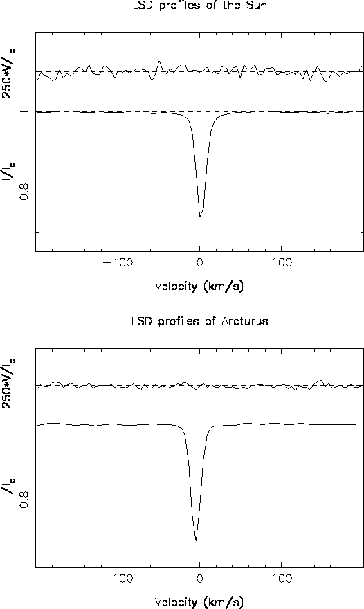Figure 7: LSD unpolarised (bottom curve of each panel) and circularly polarised (top curve of each panel) profiles, for the Sun (top panel) and Arcturus (bottom panel). Note that the LSD Stokes V spectrum are shifted upwards by 1.1 and expanded 250 times in these plots

3.1 Polarisation in line profiles

We find that the instrument performs very well for detecting polarisation in line profiles.

We first checked that no polarisation signature are detected in line profiles of slowly rotating, weakly active standard stars like the Sun or Arcturus, whose disc integrated magnetic field and associated Zeeman signatures are extremely weak. With the new LSD cross-correlation technique (Donati et al. 1997), one can extract a "mean polarisation signature'' (called LSD profile) from all recorded spectral lines simultaneously, and increase considerably the accuracy to which such polarisation signals can be detected. With such a technique, we can check for instance that no Stokes V signatures are detected on the Sun or on Arcturus down to a relative rms noise level of 0.004% and 0.002% respectively (see Fig. 7). We can conclude in particular that no spurious circular polarisation signals (due to stellar rotation and variability, Earth rotation, drifts in the spectrograph, inhomogeneities in CCD pixel sensitivities, see Donati et al. 1997, for a complete discussion) are observed for these two objects, and that our instrument, observing procedure and processing software behave correctly.

Very weak signals (with a peak-to-peak amplitude of a few 0.01%) are however detected in two LSD linear polarisation profiles of Arcturus, suggesting that the process of rotating the instrument between successive subexposures (see Sect. 2.3) probably induces systematic low level velocity shifts in the corresponding spectra (at a level of 10 to 20 ms^-1 typically) and therefore spurious polarisation signatures such as those discussed in Donati et al. (1997). Their amplitude is however sufficiently small (much smaller in particular than any of the true linear polarisation profiles we detected for the magnetic programme stars as shown below, and very often below the noise level itself) that we decided to keep using the same observing procedure (involving instrument rotations), at least till the Halle wave plate problem is fixed (see Sect. 2.3).

  

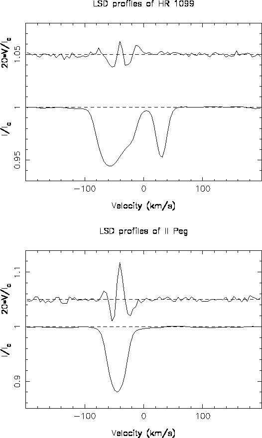Figure 8: LSD unpolarised (bottom curve of each panel) and circularly polarised (top curve of each panel) profiles of the rapidly rotating very active RS CVn systems HR 1099 (top panel) and II Peg (bottom panel), recorded on 1998 Feb. 05 and Feb. 16 respectively. The line profiles of the two system components are clearly visible in the unpolarised LSD profile of the double-line spectroscopic binary HR 1099 (K1IV+G2V) while only one line profile is visible for the single-line binary II Peg (K2IV). Note that the LSD Stokes V spectra are expanded 20 times and shifted upwards by 1.05 in these plot

The first main scientific goal of our instrument is the study of magnetic field topologies of rapidly rotating active stars through the Zeeman signatures they generate in the spectral line profiles of these objects. Figure 8 presents LSD Stokes V profiles of two of the most active RS CVn systems (HR 1099 and II Peg) obtained from MuSiCoS spectropolarimetric data recorded in 1998 February. It is obvious from these plots that Stokes V Zeeman signatures are clearly detected on both stars (with relative amplitudes of 0.12% and 0.54%, i.e. at an accuracy level of 11$\sigma$and 31$\sigma$, respectively) and are very similar in size and shape to those measured already on these stars with other instruments (Donati et al. 1992a, 1997). Note in particular that the LSD Stokes V signature of II Peg presented in Fig. 8 is the strongest ever detected on any cool stars to date. Monitoring such Zeeman signatures throughout a full stellar rotational cycle allows one to map the parent surface magnetic field topology using techniques of indirect stellar surface imaging (Doppler imaging). This new method (called Zeeman-Doppler imaging or ZDI) is found to be successful at recovering both location and shape of stellar magnetic regions as well as field strength and orientation within these regions (Donati & Brown 1997). It therefore provides a new and original way of investigating stellar dynamos in general (Donati et al. 1992b, 1998; Donati & Cameron 1997; Donati 1998). Such sets of rotationally modulated LSD Stokes V profiles have already been collected with this instrument for 4 RS CVn systems to date, the detailed analysis of which will be published in a forthcoming paper. Linear polarisation Zeeman signatures are in principle also present in spectral lines of cool active stars but are likely too weak (typically ten times weaker than their Stokes V equivalent) to be detected with our instrument.

The MuSiCoS spectropolarimeter can also be used to study the details of the magnetic topologies of magnetic chemically peculiar stars using both circular and linear Zeeman signatures which magnetic fields induce in spectral line profiles. As opposed to field topologies of active stars (consisting essentially of multiple spot distributions), field geometries of magnetic Ap/Bp stars can be described to first order as low-order axisymmetric multipole expansions. However, significant departures from such simple models (in the form of localised regions with enhanced radial field on the magnetic equator) have been detected already in several objects (e.g. Leroy et al. 1995, 1996; Wade et al. 1996). In particular, studying the nature and spatial distribution of these distortions should bring us some new insight on the still debated origin of magnetic fields in Ap/Bp stars. Unfortunately, full reconstruction of the surface magnetic topologies of such objects with no a priori assumption about their large scale structure is impossible from circular spectropolarimetry alone, as demonstrated by Brown et al. (1991). Although it is still unclear yet whether sets of rotationally modulated LSD Stokes Q and U profiles will provide the missing information for such an imaging task, it is nevertheless obvious already from Leroy et al.'s results (1995, 1996) that linear polarisation profiles in spectral lines of magnetic Ap/Bp stars will greatly improve our description of how the field topologies of these chemically peculiar stars depart from low-order axisymmetric multipole expansions.

  

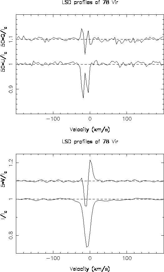Figure 9: LSD Stokes Q, U, V and I profiles (from top to bottom) of 78 Vir recorded on 1998 Feb. 18 at rotational phase 0.650 (using ephemeris JD = 2434816.90+3.7220E). Note that Stokes Q and U profiles were expanded by 50 and shifted upwards by 1.1 and 1.0 respectively, while the Stokes V spectrum is expanded by 5 and shifted upwards by 1.1 on these plots

Our instrument can successfully collect such information, as demonstrated in Fig. 9 in the particular case of the Ap star 78 Vir. The corresponding longitudinal field (estimated with the method of Donati et al. 1997) is equal to $800\pm50$ G, in good agreement with the published estimates of Borra & Landstreet (1980). Similarly, the integrated Stokes Q and U profiles we measure yield average linear polarisation angles and signs that are perfectly compatible with those determined by Leroy (1995) from broadband spectropolarimetry. It is also obvious from our observations that LSD Stokes Q and U Zeeman signatures are much more informative on the actual field structure than broadband measurements. For instance, the LSD Stokes Q profile of 78 Vir at rotational phase 0.650 is obviously non zero, although its average value implies a very weak level of broadband Stokes Q linear polarisation in agreement with the results of Leroy (1995). Similarly, MuSiCoS spectropolarimetric observations of 53 Cam at rotational phase 0.827 (i.e. when broadband measurements indicate a very low amount of linear polarisation, Leroy 1995) show that Stokes Q and U profiles, while null in average, possess a rather complex shape and should therefore be very helpful for constraining more accurately the modelling of many fine details of the surface magnetic field structure. Up to now, we have secured data sets with good to very good phase coverage for five well-known magnetic Ap stars in all Stokes parameters, whose interpretation is underway and will be published in a forthcoming paper.

  

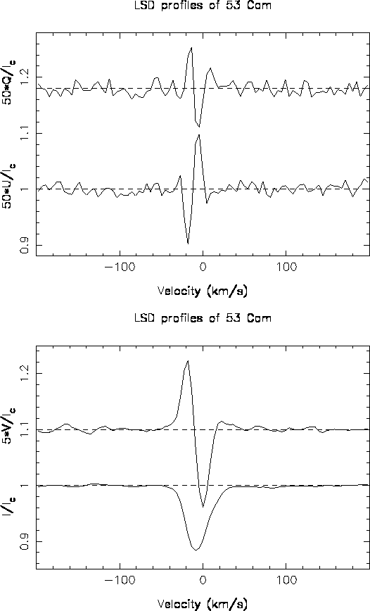Figure 10: LSD Stokes Q, U, V and I profiles (from top to bottom) of 53 Cam recorded on 1997 Feb. 25 at rotational phase 0.827 (using the new ephemeris JD = 2448500.193+8.02681E of Hill et al. 1998, with phase 0.0 referring to the positive maximum in longitudinal field). Note that Stokes Q and U profiles were expanded by 50 and shifted upwards by 1.18 and 1.0 respectively, while the Stokes V spectrum is expanded by 5 and shifted upwards by 1.1 on these plots

Finally, one can note from Figs. 9 and 10 that linear polarisation profiles are much weaker than their circular polarisation equivalent, often 15 to 20 times smaller. It is therefore very important to check for potential circular to linear polarisation instrumental crosstalk; observations of Ap stars indicate that this crosstalk rate is lower than 0.5% of the Stokes V amplitude for our polarimeter.

Other scientific applications (e.g. search for flare induced linear polarisation signatures in Balmer lines of active stars, Saar et al. 1994) should in principle be accessible to our instrument, but have not been attempted yet.

3.2 Continuum polarisation and line depolarisation structures

The MuSiCoS spectropolarimeter can in principle also estimate continuum polarisation in stellar spectra. This observing mode relies on measuring relative continuum flux variations between the two orthogonally polarised beams that correlate with wave-plate rotations. The main problem here consists in reducing true and spurious instrumental polarisation to a minimum. If the true instrumental polarisation (generated through the successive reflections onto the primary and secondary mirrors) is usually very small at the Cassegrain focus (of the order of 0.01% at TBL as estimated with the Sterenn photopolarimeter), spurious instrumental polarisation can be potentially very important. Such spurious signatures may indeed come from potential motions of the double image at fibre level (induced by wave plate rotations, instrument flexures with telescope movement or simply small random fluctuations in light injection) coupled to slight differential mispositioning of the two images onto the two fibres (due to small magnification errors in the focal reducer, to slight azimuthal misalignment of the analyser with respect to the fibre or to the chromatism of the beamsplitter).

This spurious polarisation is expected to depend only weakly on wavelength and is virtually undistinguishable from true continuum polarisation; while it is not a problem when measuring polarisation in line profiles (as we usually remove a posteriori both true and spurious continuum polarisation from the observations in this case), it can be very damaging when one is interested in studying the continuum polarisation itself, from scattering circumstellar environments for instance. As we estimate that potential mispositioning of each image onto its corresponding fibre is typically be of the order of 1 to 2 $\mu$m, we expect possible variations in the continuum flux emerging each fibre of about 2% rms and spurious polarisation levels from a sequence of four subexposures (i.e. eight spectra) of $\pm$0.7% (if the image mispositioning and associated spurious continuum flux variation does not correlate with the azimuth of the wave plate or instrument) or larger (otherwise). In practice, observations of unpolarised standard stars indicate that spurious continuum polarisation is of the order of 0.8% rms in circular polarimetry, in good agreement with the theoretical lower limit derived above. It implies in particular that wave plate rotations generate only very weak systematic image displacement at fibre input. In linear polarimetry however, the level of spurious continuum polarisation is about twice larger, indicating that the instrument rotations required in our observing procedure do produce systematic image motions at fibre input and therefore larger spurious continuum polarisation. Similarly, the accuracy to which gradients in continuum polarisation (between both edges of our spectral domain) can be estimated is typically 0.5% rms for Stokes V observations, and about twice as much for Stokes Q and U observations.

Altogether, the MuSiCoS spectropolarimeter is therefore poorly competitive at measuring stellar continuum polarisation with respect to photopolarimeters like Sterenn or Cassegrain low-resolution spectropolarimeters, which are typically two orders of magnitude more accurate for that particular purpose (e.g. Leroy 1995). This is unfortunately an intrinsic limitation of our 50 $\mu$m fibre setup.

The MuSiCoS spectropolarimeter should nevertheless be very useful for studying emission lines (and in particular, forbidden lines) depolarisation structures with respect to the surrounding continuum, and thus for determining where these lines form with respect to the scattering environment. Such depolarisation structures have for instance been recently observed in the case of the O star $\theta^1$ Ori C (see Fig. 11), at an epoch where the continuum level was circularly polarised at a rate of a few %. The fact that the emission lines of nebular origin (the [N II] lines of multiplet 1F at 654.81 and 658.36 nm, the central peak of H$\alpha$, but also the [O III] lines of multiplet 1F at 495.89 and 500.68 nm) are all depolarised in the same proportion as the line-to-continuum flux ratio indicates that all these lines are formed outside the scattering circumstellar environment and that the continuum circular polarisation is therefore of stellar (rather than interstellar) origin. A more extensive description of these results is presented in another paper (Donati & Wade 1998).

  

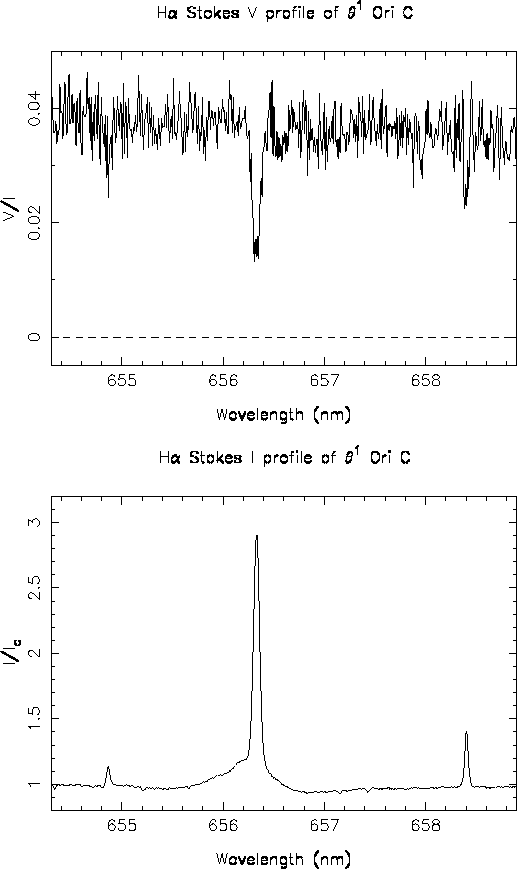Figure 11: Circular polarisation rate (top panel) and normalised intensity (bottom panel) of $\theta^1$ Ori C at H$\alpha$ wavelengths, on 1997 Feb. 20

Another potential (but yet untested) scientific application of our instrument in this field is the study of how strong winds of O stars depart from spherical symmetry through the depolarisation of spectral lines formed in the wind (Lefèvre 1992; Harries & Howarth 1996).

As continuum polarisation or line depolarisation structures produced by scattering circumstellar environments are usually an order of magnitude stronger in linear than in circular polarisation, one is usually concerned by the rate at which the instrument converts linear to circular polarisation (rather than the opposite as in Sect. 3.1). A circular analysis of 100% linearly polarised light (obtained by flat-field illumination through the linear sheet polariser located in the first polarimeter wheel, see Sect. 2.2) indicates that the crosstalk level from linear to circular polarisation is only 0.2%.