1 Introduction

ISOCAM was designed to provide images of the sky and polarization measurements in the $2.5-18~\mu$m band. It features two detectors, one for short wavelengths (SW: $2.5-5.5~\mu$m band), the other for long wavelengths (LW: $4-18~\mu$m band). The camera has two channels which cannot be used simultaneously: a selection wheel holding Fabry mirrors can direct the light beam from the ISO telescope toward either one of the detectors. The selection wheel also holds two internal calibration sources which can illuminate the detectors quasi-uniformly for flatfield purposes. In order to choose the observing configuration, there are two wheels for each channel. The first wheel holds four lenses allowing the choice of the spatial sampling: 1.5, 3, 6, and 12'' per pixel. At ISOCAM wavelengths, the spatial resolution is diffraction limited. The second wheel holds a dozen discrete band pass filters with spectral resolution ranging from 2 to 15, and continuously variable filters (CVF) with spectral resolution of 45. The sixth wheel, the entrance wheel, has four positions: one hole and three polarizers. It is possible to observe data with different exposure times (0.28, 2.1, 5.04, 6.02, 10.08, 20.16 and 60.2 s) due to the telemetry flow and on-board electronics. The electronic gain can be adjusted to 1, 2 or 4. The operating temperature of the camera is as low as 2.4 K, provided by liquid helium cooling. All details about ISOCAM, including in flight performances, are available in Cesarsky et al. (1996).

For one observation, the ISOCAM instrument delivers a set of $32\times32$frame pairs (start of integration, called Reset, and end of integration, EOI). For the long wavelength detector (LW), the signal corresponds to a simple difference between EOI and Reset. For the short wavelength detector (SW), it is more complex, and several operations such as "cross talk correction'' must be done. We assume that these corrections have been applied to the data being considered here. We have a set of data noted D(x,y,t,c): one measurement per pixel position (x,y), repeated t times, with c configurations (there is a new configuration each time the pointing position, the filter, the integration time, etc, are changed).

In the ideal case, calibration will consist of

• normalizing the data to ADU (analog-to-digital units), g^-1s^-1 by

  $$D_1(x,y,t,c) = \frac{D_0(x,y,t,c)}{gain*tint*Naccu}$$

  where gain is the electronic gain, tint is the integration time, Naccu is the number of frames already added by the on-board processing (Naccu is greater than one only in the accumulation mode, normally confined to the 0.28 second readouts (Naccu=4), or in the CAM parallel mode (Naccu=12)).
• subtract the DARK current

  $$D_2(x,y,t,c) = D_1(x,y,t,c) - {\rm dark}(x,y).$$

  The corresponding dark is extracted from the calibration library.
• divide by the optical flat (oflat) and the detector flat (dflat)

  $$D_3(x,y,t,c) = \frac{D_2(x,y,t,c)}{{\rm oflat}(x,y){\rm dflat}(x,y)}.$$

  The corresponding optical and detector flats are extracted from the calibration library.
• average the values corresponding to the same sky position and the same configuration

  $${\rm Image}(x,y,c) = {\rm mean}(D_3(x,y,1..t,c))$$

  $${\rm RMS}(x,y,c) = {\rm sigma}(D_3(x,y,1..t,c))$$

• in the case of raster observations, reconstruct the final raster map, Raster(x,y), from all images, Image(x,y,c).

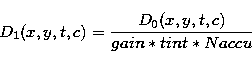
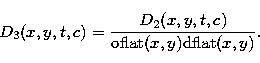
In practice, however, we have to take into account several problems:

• since the dark exhibits variation from one orbit to another, library darks obtained on specific calibration orbits are not always applicable to the data, especially at low flux.
• calibration flat fields are made with an internal source, which creates flats different from those of astronomical sources.
• cosmic rays hit the detector (see next section).
• the detector exhibits transient behavior. Each time a detector pixel is illuminated successively by a source and the background, as the detector is scanning the sky, the transition between the two flux levels is not instantaneous.
• Spacecraft jitter around the nominal pointing position randomly shifts the sources on the array during the observation.
• field of view is subject to distortion. The resolution of each pixel depends on its position in the detector.
• no signal is read from Col. 24.

Studies have been done and continue in order to resolve all of these problems, and some solutions have been proposed.

In this paper we present a selection of methods which are commonly used prior to any scientific analysis of the data. Except for the automatic flat field calculation which requires a raster mode, they can be applied to beamswitching, cvf, raster, or polarization measurements. All these methods have been naturally selected by the CAM Instrument Dedicated Team and CAM Instrument Support Team during the last two years of intensive experimentation and data reduction. Other methods also exist, but were found less efficient, or less reliable than those presented here. They are however described in the different CEA and IPAC technical reports given in the reference list.

In the calibration process proposed here, pixels are considered to be independent. This assumption is not true, due to electronic and photonic effects, and the calibration process should be considered as a first approximation. The main area in which this assumption clearly leads to incorrect results is transient correction and, to a lesser extent, cosmic ray removal.