

Up: Fabry-Perot filter based solar
Subsections
The optical layout of the video magnetograph along with the light feed is
given in Fig. 1.
![\begin{figure}
\includegraphics [width=13.9cm]{fig1.ps}
\end{figure}](/articles/aas/full/1998/20/ds1569/Timg13.gif) |
Figure 1:
Optical layout of USO video magnetograph. L1 - 15 cm objective
lens, HF - heat filter, FS - field stop, L2 - relay lens, PFW - pre-filter
wheel, KDP - KD*P
electro-optic modulator, LP - linear polarizer, FP - Fabry-Perot etalon filter,
CCD - CCD video camera, EN - Wooden enclosure |
The objective lens L1  cm, f/15 )
makes a solar image of 22 mm diameter at the focal plane where a field
stop FS is placed. A heat filter HF is used to reduce the
heat load on the optics and CCD camera saturation by blocking the IR
radiation. A portion of the image is enlarged by a factor of 2.7 by a relay lens
L2 to yield a 60 mm solar image (f/40). The pre-filter wheel
PFW, KD*P modulator, linear polarizer LP and
FP etalon filter are placed in the
telecentric beam following the lens L2. The fast axis of the
KD*P crystal makes an angle of 45
cm, f/15 )
makes a solar image of 22 mm diameter at the focal plane where a field
stop FS is placed. A heat filter HF is used to reduce the
heat load on the optics and CCD camera saturation by blocking the IR
radiation. A portion of the image is enlarged by a factor of 2.7 by a relay lens
L2 to yield a 60 mm solar image (f/40). The pre-filter wheel
PFW, KD*P modulator, linear polarizer LP and
FP etalon filter are placed in the
telecentric beam following the lens L2. The fast axis of the
KD*P crystal makes an angle of 45 with the linear
polarizer LP. Finally the image is recorded by a CCD camera.
To avoid scattered light and ambient temperature variations, all the
components are mounted on
the optical bench, and are enclosed in a wooden box EN.
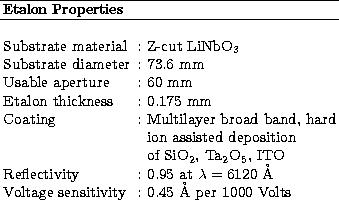
A 60 mm aperture, high finesse voltage tunable LiNbO3 FP etalon
acquired from CSIRO Australia, is used as a narrow band filter to isolate
a portion at the wing of the selected absorption line. The FP etalon is
made by using a LiNbO3 substrate of 0.175 mm thickness, both sides of
which are polished to
with the linear
polarizer LP. Finally the image is recorded by a CCD camera.
To avoid scattered light and ambient temperature variations, all the
components are mounted on
the optical bench, and are enclosed in a wooden box EN.
A 60 mm aperture, high finesse voltage tunable LiNbO3 FP etalon
acquired from CSIRO Australia, is used as a narrow band filter to isolate
a portion at the wing of the selected absorption line. The FP etalon is
made by using a LiNbO3 substrate of 0.175 mm thickness, both sides of
which are polished to  and coated with high reflective
SiO2 and Ta2O5 films. The resultant etalon has a reflectivity
of 93% over a wavelength range of 5000 to 6700 Å. The tunability of
the etalon is achieved by applying high voltage across the LiNbO3
wafer which varies its refractive index. A conductive ITO
(Indium Tin Oxide) coating is deposited for the application
of electric field across the crystal. The high voltage terminals made of
gold wires are bonded to the ITO coating with the help of silver
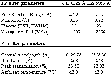
epoxy. The details of the FP parameters are given in Table 1. In
order to avoid the drift of the FP band pass due to a change in the
ambient temperature, the etalon is
enclosed in a constant temperature oven.
The oven temperature is maintained
at 43 C with a stability of
and coated with high reflective
SiO2 and Ta2O5 films. The resultant etalon has a reflectivity
of 93% over a wavelength range of 5000 to 6700 Å. The tunability of
the etalon is achieved by applying high voltage across the LiNbO3
wafer which varies its refractive index. A conductive ITO
(Indium Tin Oxide) coating is deposited for the application
of electric field across the crystal. The high voltage terminals made of
gold wires are bonded to the ITO coating with the help of silver
epoxy. The details of the FP parameters are given in Table 1. In
order to avoid the drift of the FP band pass due to a change in the
ambient temperature, the etalon is
enclosed in a constant temperature oven.
The oven temperature is maintained
at 43 C with a stability of  0.05 C which
provides a wavelength stability 5 mÅ. A bench test was performed
for determining different parameters of the FP etalon, by placing it
in front of the USO Littrow spectrograph coupled with 15 cm Zeiss
coudé telescope. This spectrograph has a dispersion of 0.047 Å/pixel
and an f-ratio of f/40 similar to the light beam used for the video magnetograph.
Figure 2a show the observed FP channel spectrum recorded near CaI
6122 Å.
0.05 C which
provides a wavelength stability 5 mÅ. A bench test was performed
for determining different parameters of the FP etalon, by placing it
in front of the USO Littrow spectrograph coupled with 15 cm Zeiss
coudé telescope. This spectrograph has a dispersion of 0.047 Å/pixel
and an f-ratio of f/40 similar to the light beam used for the video magnetograph.
Figure 2a show the observed FP channel spectrum recorded near CaI
6122 Å.
![\begin{figure}
\includegraphics [height=6cm]{fig2a.ps}
\includegraphics [height=6cm]{fig2b.ps}
\end{figure}](/articles/aas/full/1998/20/ds1569/Timg17.gif) |
Figure 2:
The observed and corrected Fabry-Perot channel spectra:
a) and b) show the observed and corrected channel spectra at
6122 Å. The dotted line shows the solar spectrum, the intensity is
plotted in arbitrary units |
The observed profiles are corrected for the spectrograph instrumental
broadening, using the CaI
6122 Å line profile obtained from KPNO digital solar spectral atlas
(Debi et al. 1998). The corrected profile is shown in
Fig. 2b. At H 6563 Å also, the results are similar.
Solar spectra were recorded by removing the FP etalon placed in front of the
spectrograph slit. The measured Full-width at half maximum (FWHM),
Free-Spectral range (FSR), and finesse (FSR/FWHM) of the etalon are given
in the Table 1. The voltage tunability of the etalon was determined
by measuring the wavelength shift of the channel spectrum as a function of
voltage in the range of -3000 to + 3000 Volts in steps of 50
Volts. With in this range the wavelength shift is linear with voltage and is
found to 0.45 Å per 1000 Volts.
6563 Å also, the results are similar.
Solar spectra were recorded by removing the FP etalon placed in front of the
spectrograph slit. The measured Full-width at half maximum (FWHM),
Free-Spectral range (FSR), and finesse (FSR/FWHM) of the etalon are given
in the Table 1. The voltage tunability of the etalon was determined
by measuring the wavelength shift of the channel spectrum as a function of
voltage in the range of -3000 to + 3000 Volts in steps of 50
Volts. With in this range the wavelength shift is linear with voltage and is
found to 0.45 Å per 1000 Volts.
To isolate 6122 Å (CaI) and 6563 Å (H) lines two narrow
band interference filters of passband 2.6 Å and 3.5 Å respectively
are placed before the FP, and the voltage on the FP is accordingly changed
to obtain VMG in 6122 Å line and H filtergrams.
These two pre-filters are also enclosed in separate temperature controlled
ovens and mounted on computer controlled filter wheel, in order to make
near simultaneous magnetic field, chromospheric, and photospheric observations.
Table 1:
Narrow band filter parameters
| |
A KD*P electro-optic quarter wave plate and a linear polarizer constitute
the circular polarization analyzer for measuring the longitudinal
magnetic field.
The modulator uses a thin (< 3 mm) Meadowlark KD*P
crystal which makes these cells suitable for using them in convergent
light beam
slower than f/20 (West 1989). The fast axis of the
KD*P crystal
is aligned at 45 to the transmission axis of the linear
polarizer and housed in an insulated enclosure. The KD*P crystal is
converted to  retarders (at
  Å)
by applying
Å)
by applying  Volts. In order to operate the KD*P modulator
a fast switchable high voltage power supply was made, which can provide
Volts on the application of low voltage TTL pulses at the
input. The TTL pulses are obtained from the centronics port of the image
acquisition system and synchronized with the image frame acquisition,
such that alternately captured video frames contain left or right
circularly polarized images. The left and right circular Zeeman
components are converted in to two mutually perpendicular linear
polarizations depending on the sign of the applied voltage. One of the
components is blocked by the linear polarizer allowing the selection of
the image corresponding to left or right
circular polarization in the emerging beam.
The detector used in the video magnetograph is a Cohu make CCD monochrome
camera with image sensor chip TC277
from Texas Instruments. This camera provides high resolution images with
sensitivity as low as 0.25 lux, zero geometric distortion and no lag or
retention of images. The CCD used is a frame transfer device with
Volts. In order to operate the KD*P modulator
a fast switchable high voltage power supply was made, which can provide
Volts on the application of low voltage TTL pulses at the
input. The TTL pulses are obtained from the centronics port of the image
acquisition system and synchronized with the image frame acquisition,
such that alternately captured video frames contain left or right
circularly polarized images. The left and right circular Zeeman
components are converted in to two mutually perpendicular linear
polarizations depending on the sign of the applied voltage. One of the
components is blocked by the linear polarizer allowing the selection of
the image corresponding to left or right
circular polarization in the emerging beam.
The detector used in the video magnetograph is a Cohu make CCD monochrome
camera with image sensor chip TC277
from Texas Instruments. This camera provides high resolution images with
sensitivity as low as 0.25 lux, zero geometric distortion and no lag or
retention of images. The CCD used is a frame transfer device with
 m
pixels arranged in
m
pixels arranged in  array in which half of the pixel
rows are masked for image storage and the other half are exposed to light.
This makes a resultant image area of
array in which half of the pixel
rows are masked for image storage and the other half are exposed to light.
This makes a resultant image area of  mm on the CCD
chip. CCIR scanning system is employed for the image read out, where a
single video field (one video frame contains two video fields -odd and
even) takes 1/50 seconds for scanning. During every video field the charge
accumulated in the storage section is read out while the image section is
exposed. The vertical blanking pulses after each video field
(two vertical blanking pulses for each video frame) in the CCIR video
output is detected through software and used for the synchronization of
the KD*P switching and the entire data acquisition and reduction
process. In the present optical set-up an area of
mm on the CCD
chip. CCIR scanning system is employed for the image read out, where a
single video field (one video frame contains two video fields -odd and
even) takes 1/50 seconds for scanning. During every video field the charge
accumulated in the storage section is read out while the image section is
exposed. The vertical blanking pulses after each video field
(two vertical blanking pulses for each video frame) in the CCIR video
output is detected through software and used for the synchronization of
the KD*P switching and the entire data acquisition and reduction
process. In the present optical set-up an area of  arcmin of the solar disk is imaged by the camera, which gives a
resolution of
arcmin of the solar disk is imaged by the camera, which gives a
resolution of  arcsec/pixel.
Block diagram of the image acquisition and control system of the
video magnetograph is given in Fig. 3.
arcsec/pixel.
Block diagram of the image acquisition and control system of the
video magnetograph is given in Fig. 3.
![\begin{figure}
\includegraphics [height=10cm]{fig3.eps}
\end{figure}](/articles/aas/full/1998/20/ds1569/Timg27.gif) |
Figure 3:
The schematic diagram of the optics, image acquisition system and
control electronics |
An Innovision Inc., workstation, based on Motorola, MC68030,
single board VMEbus computer, and integrated with Imaging Technology
Series 150 image processing modules makes the complete data acquisition
and control system. The image processing modules consists of one
analogue-to-digital interface (ADI) unit, two frame buffers (FB) and one
arithmetic and logic unit (ALU); all connected to the VMEbus of the host
computer. The combination of the host computer, series 150 modules and
suitable software
can perform complex on-line real time digital image processing tasks such
as averaging of images and subtraction. The ADI employs an 8-bit flash
A/D converter at 10 MHz
sampling rate, which digitizes the video input signal to 256 gray levels.
The video bus transmits the digitized data (VDI) to all the other modules.
The frame buffers FB0 and FB1 contains the image storage required
for the real time processing of the data. Each FB consists of a single
512 by 512 by 16-bit frame store (FRAME A) and two 512 by 512 by 8-bit
frame stores (B1 and B2). ALU is a pipelined image processor which
provides real time image processing capabilities when used with ADI and FB.
The images from FRAME A and FRAME B are processed by ALU and the result is
stored in FRAME A, which is finally transferred to the host computer.
A software was developed using C-language and ITEX 150/151 image processing
library (Imaging Tech, Inc) for real time processing and control of the
video magnetograph (Mathew 1998). The flow chart
illustrates the sequence of operation performed by the software during a
single acquisition cycle (Fig. 4a).
![\begin{figure}
\centering
\includegraphics [width=16.5cm]{fig4ab.ps}
\end{figure}](/articles/aas/full/1998/20/ds1569/Timg28.gif) |
Figure 4:
Flow chart showing: a) the operations involved in a
single cycle of image acquisition, b) VMG operation for a single video
magnetogram |
The centronics port data bits D0 to D5, performs
various control operations such as opening and closing the telescope
shutter, changing the pre-filter, moving the relay lens for focusing the image
for H and CaI, changing the polarizer wheel, and
switching the KD*P high voltage supply. A single acquisition cycle
consists of several operations to obtain selected number of magnetograms,
CaI 6122 Å and H images. To obtain the
photospheric CaI 6122 Å images, the filter is kept tuned at the
same position where the Stokes V signal is taken.
The flow chart
in Fig. 4b shows various steps involved to obtain a single
video magnetogram.
For making magnetograms, the Series150 modules are set up for continuous
acquisition
and adding up of the images. The ALU is programmed for adding the
incoming video
data on to the pervious image already present in the FRAME A.
The alternate incoming video images are routed to FRAME A of FB0 and FB1
respectively. This is synchronized with the KD*P high voltage switching
such that the alternate frames are taken in the left and right circular
polarizations. This process can be repeated for a pre-selected number of
frames (maximum of 256 frames) to increase the signal to noise (S/N) ratio.
To integrate 256 frames, the systems takes 12 seconds.
The whole sequence of one observation, takes about 1 minute which
consists of a video magnetogram averaged over 256 frames,
CaI photospheric image and H filtergram.
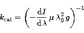
The calibration of the video magnetograms were made by using the profile line
slope method (Varsik 1995), which is based on the weak
field approximation (Jefferies & Mickey 1991).
The Stokes parameter V can be expressed as,
|  |
(2) |
|  |
(3) |
where  mc2; e and m are the charge and mass
of the electron,
mc2; e and m are the charge and mass
of the electron,  the central wavelength of observation in
Å, g the Landé factor of transition for absorption line,
B|| is the longitudinal magnetic field in Gauss and
the central wavelength of observation in
Å, g the Landé factor of transition for absorption line,
B|| is the longitudinal magnetic field in Gauss and  is the calibration factor. I the Stokes
intensity obtained in the absence of magnetic field and V is the
intensity obtained by subtracting a single pair of video frames taken
in opposite circular polarization. dI/d
is the calibration factor. I the Stokes
intensity obtained in the absence of magnetic field and V is the
intensity obtained by subtracting a single pair of video frames taken
in opposite circular polarization. dI/d is the measured line
slope by tuning the filter from - 40 mÅ to -170 mÅ from
the line center in the steps of 25 mÅ.
The measured slope
dI/d is found to be 0.047, which gives the value of
is the measured line
slope by tuning the filter from - 40 mÅ to -170 mÅ from
the line center in the steps of 25 mÅ.
The measured slope
dI/d is found to be 0.047, which gives the value of
 using Eq. (3). This constant is used in Eq. (2)
for conversion of measured Stokes V intensity into the magnetic
field values in Gauss. The measured longitudinal magnetic field is the
observed average field over the spatial resolution element and limited
by the solar seeing. Further as the spectral resolution of the FP etalon
is small, the accuracy of calibration by this method is rather low.
using Eq. (3). This constant is used in Eq. (2)
for conversion of measured Stokes V intensity into the magnetic
field values in Gauss. The measured longitudinal magnetic field is the
observed average field over the spatial resolution element and limited
by the solar seeing. Further as the spectral resolution of the FP etalon
is small, the accuracy of calibration by this method is rather low.
Figures 5a and b show USO and SOHO/MDI video magnetograms obtained
around the same time on 09 April 1997.
![\begin{figure}
\includegraphics []{fig5ab.ps}
\end{figure}](/articles/aas/full/1998/20/ds1569/Timg35.gif) |
Figure 5:
The magnetograms obtained for comparison on 09 April 1997
by: a) USO video magnetograph at 09:32 UT, b) SOHO/MDI at 09:41
UT |
The SOHO/MDI magnetogram is a part of the
calibrated full-disk data (Scherrer et al. 1995). It
may be noticed that all the features observed in both the video
magnetograms match well. After accurate registration of the two VMGs and
degrading the spatial resolution of USO VMG to
match the SOHO/MDI, a scatter diagram has been plotted and shown in
Fig. 6.
![\begin{figure}
\includegraphics [height=9cm]{fig6.ps}
\end{figure}](/articles/aas/full/1998/20/ds1569/Timg36.gif) |
Figure 6:
Scatter plot made between calibrated USO and SOHO magnetograms |
![\begin{figure}
\includegraphics []{fig7ab.ps}
\end{figure}](/articles/aas/full/1998/20/ds1569/Timg37.gif) |
Figure 7:
A typical: a) video magnetogram and b) CaI
6122 Å (-140 mÅ) image |
![\begin{figure}
\includegraphics []{fig8.ps}
\end{figure}](/articles/aas/full/1998/20/ds1569/Timg38.gif) |
Figure 8:
Composite picture of magnetogram, CaI 6122 Å (-140 mÅ) and H
images showing one cycle multi-wavelength observation. The upper panel shows
the images of active region NOAA#7843 taken on 19 February 1995 and the lower
panel shows the same active region on 20 February 1995 |
This plot demonstrate the
validity of the calibration procedure, except for a small deviation of
the slope of the scatter line from unity. This deviation may be attributed
to the use of different spectral lines and difference in spectral and spatial
resolution of the two instruments.
Up: Fabry-Perot filter based solar
Copyright The European Southern Observatory (ESO)
![\begin{figure}
\includegraphics [height=6cm]{fig2a.ps}
\includegraphics [height=6cm]{fig2b.ps}
\end{figure}](/articles/aas/full/1998/20/ds1569/img17.gif)
![\begin{figure}
\includegraphics [height=10cm]{fig3.eps}
\end{figure}](/articles/aas/full/1998/20/ds1569/img27.gif)