2 Theory

2.1 Target wavefunctions

The lowest eleven states of the target ion, i.e., 3s, 3p, 3d, 4s, 4p, 4d, 4f, 5s, 5p, 5d and 5f states, are included in the present calculation. Each state is represented by a configuration interaction wavefunction. The radial part of the one-electron orbitals is expressed in the Slater form

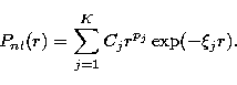$$P_{nl}(r) = \sum_{j=1}^{K} C_{j}r^{p_{j}}\exp(-\xi_{j}r).$$ (1)

The coefficients C_j and the parameters p_j and $\xi_{j}$ for the 1s, 2s, 2p and 3s orbitals are taken from the paper by Clementi & Roetti (1974), while those for the other orbitals are obtained with the computer code of Hibbert (1975) by optimizing those orbitals on the energy of the corresponding states.

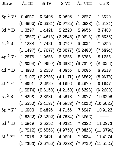
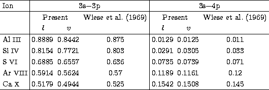
Excitation energies obtained in the present calculation are compared in Table 1 with the experimental results (Moore 1971). The excitation energies of Ar VIII are different from those of the Paper I owing to the use of 3d orbital with three terms. Oscillator strengths for the optically allowed transitions from the ground state to 3p and 4p states are shown in Table 2. Both the excitation energies and the oscillator strengths obtained in the present calculation are in good agreement with those of experiment and those of other calculations. This indicates the reliability of the present wavefunction of the target ions.

  

Table 1: Excitation energies (in Ryd) from the ground state of the Na-like ions: comparison of the present calculation and the observed values from Moore (1971) (in parentheses)

  

Table 2: Oscillator strengths

2.2 Collision calculations

The R-matrix theory of electron-ion collisions has been described in detail by Burke & Robb (1975). The total wavefunction representing the electron-ion collision system is expanded in a sphere with radius $r_{\rm a}$ as follows:

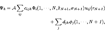$$\begin{eqnarray} \Psi_{k} = {\cal A} \sum_{ij}c_{ijk}\Phi_{i}(\rm 1,\cdot\cdot\c... ...onumber \\ +\sum_{j}d_{jk}\phi_{j}(\rm 1,\cdot\cdot\cdot,\it N+1),\end{eqnarray}$$ (2)

where $\cal A$ is the anti-symmetrization operator, $\Phi_{i}$ the channel function representing the target state coupled with the spin and angular functions for the scattering electron, u_ij the continuum basis orbitals for the scattered electron, and $\phi_{j}$ twelve-electron bound configurations formed from fourteen bound orbitals. Details of the basis functions u_ij and $\phi_{j}$ are described in Paper I. The coefficients c_ijk and d_jk are determined by diagonalizing the total Hamiltonian of the whole system with the basis set expansion defined by Eq. (2).

We use the computer code of Berrington et al. (1978) to calculate the R-matrix on the boundary of the sphere, whose radius ($r_{\rm a}$) is taken to be 27.8, 21.0, 14.2, 11.0 and 8.8 a.u. for Al III, Si IV, S VI, Ar VIII and Ca X, respectively. We include 30 continuum orbitals for each ion. In the outer region of the sphere, a set of close-coupling equation is solved for the partial waves L = 0-10, using the asymptotic code STGF of Berrington et al. (1987). Contributions from the partial waves higher than those are evaluated by using a two-state close-coupling approximation of Henry et al. (1981) and the Coulomb-Born approximation of Takagishi et al. (1995).

2.3 Calculation of rate coefficients

Excitation rate coefficients C(in cm³ s^-1) for a transition i to f is calculated using the following formula,

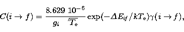$$C(i\rightarrow f) = \frac{ 8.629\ 10^{-6}}{{g_{i}\ \sqrt{T_{... ...}}}} \exp\it(-\Delta E_{if}/kT_{\rm e})\gamma(i\rightarrow f),$$ (3)

where ${\gamma}$ is the effective collision strength defined by

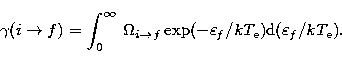$$\gamma(i \rightarrow f) = \int_0^{\infty}\,\Omega_{i\rightar... ..._{f}/kT_{\rm e}) \rm d\it({\large \varepsilon}_{f}/kT_{\rm e}).$$ (4)

Here ${\large \varepsilon}$_f is the energy of the electron after the collision, g_i the statistical weight of the level $i , \ \Delta E_{if}$ the excitation energy, and $\Omega_{i\rightarrow f}$the collision strength. The temperature $T_{\rm e}$ is expressed in K. To obtain the rate coefficient at high temperature, we fit the present collision strengths in the region where no resonances appear to an analytic form  

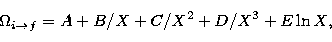$$\Omega_{i\rightarrow f} = A + B/X + C/X^{2} + D/X^{3} + E\ln X,$$ (5)

where X = k²_i/$\Delta E_{if}$, where k²_i is the incident energy in Ryd and $\Delta E_{if}$ is given in Ryd. For a dipole-allowed transition, the form is used with D = 0 and E = 4g_if_if/$\Delta E_{if}$, where f_if is the oscillator strength for $i\rightarrow f$.The form (5) with E = 0 is used for optically forbidden cases. Thus the effective collision strength is evaluated with the collision strengths calculated in the resonance region and with the Eq. (5) otherwise.