2 Parameter set and objective function

2.1 Parameter set

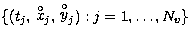
Suppose we have three sets of measurements, namely

1.

$\{ (t_j,\,{\stackrel{\rm \circ}{x}}_j,\,{\stackrel{\rm \circ}{y}}_j): j=1,\dots,N_v \}$: a set of measured relative rectangular coordinates of the fainter (B) with respect to the brighter (A) component

2.

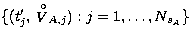$\{ (t'_j,\,{\stackrel{\rm \circ}{V}}_{A,j}): j=1,\dots,N_{s_A}\}$: a set of radial velocity measurements for the spectroscopic component A

3.

$\{(t{''}_j,\,{\stackrel{\rm \circ}{V}}_{B,j}): j=1,\dots,N_{s_B}\}$: a set of radial velocity measurements for the spectroscopic component B

for a double-lined spectroscopic visual binary. We reckon with radial velocities expressed in km s^-1 and positions in arcsec ('').

For the visual orbit, we have

$$\begin{eqnarray} x&=&AX+FY\\ y&=&BX+GY\\ X&=&\cos E-e\\ Y&=&\sqrt{1-e^2}\sin E,\end{eqnarray}$$ (1) (2) (3) (4)

where X and Y (x and y) are the angular rectangular coordinates, in the orbital (tangential) plane, of the fainter component with respect to the brighter one; A, B, F and G are the Thiele-Innes constants, expressed in terms of a(''), i, $\omega$ and $\Omega$ as

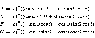$$\begin{eqnarray} A&=&a{('')}(\cos\omega\cos\Omega-\sin\omega\sin\Omega\cos i)\\ ... ...)\\ G&=&a{('')}(-\sin\omega\sin\Omega+\cos\omega\cos\Omega\cos i).\end{eqnarray}$$ (5) (6) (7) (8)

e is the eccentricity and E is eccentric anomaly, determined unambiguously by Kepler's equation

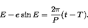$$E-e\sin E=\frac{2\pi}{P}(t-T).$$ (9)

P is the period and T is the epoch of periastron passage. Seven parameters (a(''), i, $\omega$, $\Omega$, e, P and T) are necessary.

For a spectroscopic orbit j (j=A or j=B) , we have

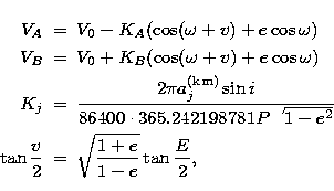$$\begin{eqnarray} V_A&=&V_0-K_A(\cos(\omega+v)+e\cos\omega)\\ V_B&=&V_0+K_B(\cos(... ...1-e^2}}\\ \tan\frac{v}{2}&=&\sqrt{\frac{1+e}{1-e}}\tan\frac{E}{2},\end{eqnarray}$$ (10) (11) (12) (13)

where again the symbols have their usual meaning.

We switch from the angular separation to the linear one using

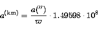$$a^{\rm (km)}=\frac{a{('')}}{\varpi}\cdot 1.49598\cdot 10^{8}$$ (14)

where $\varpi$ is the parallax of the system. By introducing $\kappa$, the ratio of a_A to a_A+a_B, we can now write

$$\begin{eqnarray} a_A^{\rm (km)} &=&\kappa a^{\rm (km)}\\ a_B^{\rm (km)}&=&(1-\kappa)a^{\rm (km)}.\end{eqnarray}$$ (15) (16)

The system as a whole thus needs the following ten parameters for its complete specification:

• a(''): the semi-major axis of the relative orbit of the faintest component around the brightest star;
• i: the inclination of the orbital plane with respect to the plane orthogonal to the sight direction;
• $\omega$: the argument of the periastron;
• $\Omega$: the longitude of the ascending node;
• e: the eccentricity;
• P: the period;
• T: the periastron epoch (one of them);
• V₀: the radial velocity of the system's center of mass;
• $\varpi$: the parallax of the system;
• $\kappa$: the ratio of the semi-major axis (relative to the brighter component) to the sum of the two semi-major axes.

With these parameters, we face a problem of constrained minimization because $e\in [0,1[$ while $\varpi\in ]0,1[$ and $\kappa\in ]0,1[$.

Other parameter sets are actually possible (e.g., by introducing K_A and K_B, the amplitude of the radial velocity curves, the mass ratio, ...). However, we do not believe one is systematically better than another. Starting from the orbital parameters of visual binaries, the extension with V₀, $\varpi$ and $\kappa$ seems natural to us.

One could be tempted to use the variable transformation proposed by Soulié (1986) to convert a constrained minimization problem into an unconstrained one (or, at least, a less constrained one). Soulié's variable transformation is:

$$x=\frac{x'^2}{1+x'^2},$$

where x is a variable in [0,1[ and $x'\in R$. This could be applied to e, $\varpi$ and $\kappa$. Unfortunately, this makes the system even more nonlinear than it already is (the condition number of the objective function increases). We noticed that starting from a uniform distribution of x', we do not get a uniform distribution of x. We therefore decided to keep the problem in its constrained version. We managed the constraints by returning a huge value for the objective function when one of the constraints is not satisfied.

2.2 The objective function

We are looking for a function that attains its minimum at the best estimate for the orbital parameters. This function has to allow one to combine visual measurements (in the current state of our work, only Cartesian coordinates (in the tangential plane)) and radial velocities. We assume that x and y are observed at the same time, but we assume nothing about the observation time of the three data sets. In fact, we treat these three sets independently.

Assume that none of the observations are correlated and choose the objective function as

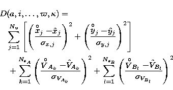$$\begin{eqnarray} \lefteqn{D(a, i, \dots, \varpi, \kappa)=}\nonumber\\ &&\sum_{j=... ...krel{\rm \circ}{V}_{B_l}-\hat{V}_{B_l}}{\sigma_{V_{B_l}}}\right)^2\end{eqnarray}$$ (17)

where the hat (super) stands for the adjusted (observed) quantity.

D satisfies the mathematical and statistical requirements for a least-squares adjustment Eichhorn (1993). Equation (17) can be rewritten as

$$D(a, i, \dots, \varpi, \kappa)=\mbox{\boldmath$\xi$}^{\mathrm{T}}\mbox{\boldmath$\Sigma$}^{-1}\mbox{\boldmath$\xi$}$$

where $\xi$ is a 2N_v+N_sA+N_sB-vector composed of $\stackrel{\rm \circ}{x}-\hat{x}$, $\stackrel{\rm \circ}{y}-\hat{y}$, $\stackrel{\rm \circ}{V}_A-\hat{V}_A$ and $\stackrel{\rm \circ}{V}_B-\hat{V}_B$ and $\Sigma$ is a diagonal matrix composed of $\sigma_x$, $\sigma_y$, $\sigma_{V_A}$, $\sigma_{V_B}$, the variances of the observed quantities in the appropriate order.