4 Density and luminosity functions

The procedure described in the previous Sect. 3 is illustrated in Figs. 3-5, where the density functions (histograms) for the different population types are given for stars of different absolute magnitudes. In each panel, the observed densities are represented by model curves (i.e., density gradients) which were calculated from the density laws adopted for the corresponding population components by Gilmore & Wyse (1985) and which were then fitted to the data at the centroid distances of their corresponding volumes (full dots) by least-squares. Note that the intersections of these fits with the ordinates provide the estimates of the local luminosity function extrapolated from the observations.

  

Figure 3: Histograms of logarithmic space densities as functions of absolute magnitude (panels) for all population components combined. Curves are model density gradients from Gilmore & Wyse (1985) fitted to the observations at centroid distances (dots) within survey completeness limits (arrows) by least squares. Their intersections with the ordinates (r=0) provide the extrapolated local densities

  

Figure 4: Luminosity function resulting from observed local densities extrapolated in Fig. 3 (dot-dashed line). Comparison with the luminosity function derived from the Catalog of Nearby Stars by Gliese (1969) indicates that the initial two-color classification of the stars is likely biassed by assuming too many unevolved main sequence stars at faint absolute magnitudes

  

Figure 5: Histograms of logarithmic space densities as functions of absolute magnitude for the intermediate (left) and the extreme (right) population II components. Solid curves are model density gradients from Gilmore & Wyse (1985) which, if fitted to the observations as in Fig. 3 (dashed), show that the steeper observed gradients also imply excess extrapolated local densities

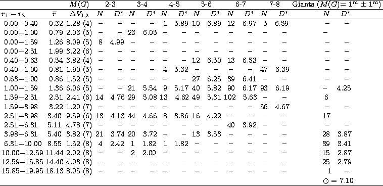
Results of the original trial are shown for the density profiles summed over all three population components in Fig. 3. It is gratifying to see that for the full range of absolute magnitudes and within the completeness limits of the survey (indicated by the vertical arrows) there is good qualitative agreement between the observed and the model-predicted density gradients. However, the corresponding extrapolated local densities (i.e., at r=0) yield a luminosity function which is significantly different from the Gliese standard, as displayed in Fig. 4. Obviously, the present data show a significant excess of intrinsically fainter stars (M_G>6) which seems to be balanced by a strong apparent deficiency of intrinsically brighter stars (M_G<5).

Now, inspection of Fig. 5 immediately tells us that the apparent excess of nearby stars is most likely due to the (expected) bias in the absolute magnitudes assigned to the alleged intermediate and extreme population II stars: their observed density gradients are all much steeper than predicted by the model, leading to extrapolated local densities which are too high relative to the model standard by up to more than two orders of magnitude for the fainter stars, M_G>6. Thus, the most straightforward - and, in fact, plausible - explanation is that a substantial fraction of these excess nearby stars should be redistributed to the larger distances implied by brighter absolute magnitudes, M_G<4. Also note that stars of these lower-metallicity population components which have absolute magnitudes M_G<5 cannot be main sequence stars but must be evolved to near or beyond the turnoff, even if they should have relatively young ages, >5 Gyr (BF90); therefore, density profiles for the brighter main sequence stars of these population components are naturally lacking in Fig. 5.

Thus, based on the differences between the luminosity functions of Fig. 4, and depending on the individual observed density histograms and excesses indicated in Fig. 5, between 30% and 60% (for an average of $\sim$$43\%$) of the relatively nearby intermediate and extreme population II stars were (randomly) selected in each of the three absolute magnitude intervals (M_G>5) for reassignment of their M_G in a first iteration cycle. For each star, the theoretical CMD given by BF90 was used again for substituting for the former main-sequence luminosity the brighter absolute magnitude corresponding to the more advanced evolutionary stage near the turnoff or the subgiant branch associated with its same observed G-R color, $\delta_{U{-}G}$-derived metallicity-class, and adopted (old-)age isochrone, as in the previous cycle.

  

Table 1: Logarithmic space densities for Population I stars: $D^{*}=\log D+10$, where $D=N/\Delta V$, and where N is the number of stars in the partial volume $\Delta V_{1,2}= (\pi/180)^{2}(\ifmmode\hbox{\rlap{$\sqcap$}$\sqcup$}\else{\unsk... ...up$} \parfillskip=0pt\finalhyphendemerits=0\endgraf}\fi/3)(r_{2}^{3}-r_{1}^{3})$ with field-size $\ifmmode\hbox{\rlap{$\sqcap$}$\sqcup$}\else{\unskip\nobreak\hfil \penalty50\hsk... ...box{\rlap{$\sqcap$}$\sqcup$} \parfillskip=0pt\finalhyphendemerits=0\endgraf}\fi$(in square degrees), limiting distances r₁ , r₂, and centroid distance $\overline{r}=[(r^{3}_{1}+r^{3}_{2})/2]^{1/3}$.Distances are in kpc, volumes in $\rm pc^{3}$

  

Table 2: Logarithmic space densities for Intermediate Population II stars. Symbols as in Table 1

  

Table 3: Logarithmic space densities for Extreme Population II stars. Symbols as in Table 1

  

Table 4: Logarithmic space densities for all population components combined. Symbols as in Table 1

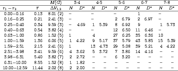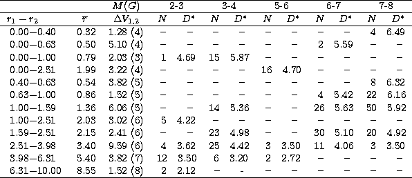
Results of this first - and only - iteration are given in Tables 1-5 and illustrated in Figs. 6-9 to show that a consistent (although not proven unique) solution can be readily found by this simple procedure. Most density histograms for the population II components derived from the alternative absolute magnitude determinations and displayed in Fig. 6 do indeed follow well the flatter predicted gradients throughout the ranges set by the completeness limits of the survey. The same also holds for the profiles combining the contributions of all three population components in Fig. 7, which yield an (extrapolated) local luminosity function (Fig. 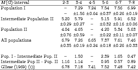8) that is now fully consistent with the adopted reference standard! Note that, relative to the population I stars, the local densities extrapolated from the panels of Fig. 6 for the intermediate and the extreme populations II also agree fairly well, on average, with the independent (i.e., canonical) values of $\sim$$3\%$ and $\sim$$0.1\%$,respectively (cf. Buser et al. 1998a). The large variation given in Table 5 (lines 4 and 10) for the intermediate population II at 5<M_G<8 is due partly to the coarseness of the present method, partly to the intrinsic difficulty to separate these faint main sequence dwarfs from the population I red giants which occupy the same area (G-R > $\sim 1.2$) in the two-color diagram. Still, for a total of 131 red giants (of population I) that were identified in the present sample, the density profile shown in Fig. 9 is in excellent agreement with the model prediction, and the extrapolated local density given in Table 4 (D^*₀=7.10) again closely matches the standard (D^*₀=6.92) provided by Gliese & Jahreiss (1992). However, since the local density of red giants as derived from HIPPARCOS data may be lower by almost a factor of two (Jahreiss & Wielen 1997), the above result has been somewhat weakened as a constraint to the present analysis.

  

Figure 6: Histograms of logarithmic space densities as functions of absolute magnitude for the intermediate (left) and the extreme (right) population II components, after assignment of turnoff- and subgiant luminosities ($2<M_{G}\leq 4$) to a selected number of lower-metallicity class stars initially assumed to be on the main sequence ($5<M_{G}\leq 8$). Note that, in general, the gradients now agree better with the model fits (curves), as do the corresponding extrapolated local densities (see the text)

  

Figure 7: Histograms of logarithmic space densities as functions of absolute magnitude for all population components combined, after assignment of turnoff- and subgiant luminosities ($2<M_{G}\leq 4$) to a selected number of lower-metallicity class stars initially assumed to be on the main sequence ($5<M_{G}\leq 8$). Note that, in general, the gradients now agree better with the model fits (curves), as do the corresponding extrapolated local densities (see the text)

  

Figure 8: Luminosity function resulting from observed local densities extrapolated in Fig. 7 (dotted line). Obviously, the Gliese standard (solid line) has been successfully used as a constraint in the first iteration of the present analysis. The disagreement at MG=4.5 is a feature germane to old metal-poor populations (see the text)

  

Figure 9: Density profile for late-type population I red giants identified in the two-color diagrams of the present field. The observed gradient and the extrapolated local density agree well with the model prediction and the Gliese-Jahreiss (1992) standard, respectively (see the text)

Note also that the observed dip at M_G=4.5 in Fig. 8 does not disturb the agreement with the standard but is consistent with theoretical expectations: because the evolutionary tracks and isochrones become increasingly vertical near this absolute magnitude in the CMD for old metal-poor populations, the more rapid evolutionary phases away from the main sequence and through the turnoff "dilute" their original main-sequence luminosity function (i.e., IMF) into a broader absolute magnitude range which leads to significant depletion of stars at some characteristic magnitude of their present-day luminosity function, to a larger uncertainty in the determination of individual absolute magnitudes, and to accordingly modified associated Malmquist corrections (Gilmore 1984). In fact, the feature has been observed prominent in far-field stellar samples away from the Galactic plane, because due to their greater average ages relative to the normal (thin) disk, these stars also have larger scale heights resulting from their prolonged post-collapse dynamical evolution (Wielen 1974).

  

Table 5: Local densities and their standard deviations, $D^{*}_{0}\pm \sigma_{D^{*}_{0}}$, extrapolated from observed density profiles by least-squares. The three bottom lines include the local-density differences between population components, and, for comparison, the Gliese standard