In this section we briefly present the basic issues for generating high resolution full sky maps which include CMB fluctuations and the galactic emission.
The CMB anisotropy is usually written as
(Bond & Efstathiou 1987;
White et al. 1994):
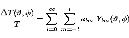 |
(1) |
 |
(2) |
![\begin{eqnarray}
\frac{\Delta T(\vartheta,\phi)} {T} =&&
\sum_{l=2}^{
\l
_{\r...
...\nonumber \\ &\times & \cos(m\phi)- \Im m (a_{lm}) \sin(m \phi) ].\end{eqnarray}](/articles/aas/full/1998/12/ds7256/img9.gif) |
||
| (3) |
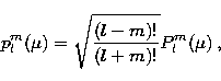
In Eq. (3)
only the polynomials plm
depend on ![]() , while all
the dependence on
, while all
the dependence on ![]() is in the square bracket part.
This particular feature makes the choice of the pixelisation (i.e. the
set of
is in the square bracket part.
This particular feature makes the choice of the pixelisation (i.e. the
set of ![]() where to calculate
where to calculate ![]() ) a
crucial parameter for the computational cost of the simulation.
The "standard'' COBE-cube pixelisation satisfies
two simple symmetry properties:
1) if
) a
crucial parameter for the computational cost of the simulation.
The "standard'' COBE-cube pixelisation satisfies
two simple symmetry properties:
1) if ![]() ,
then
also
,
then
also ![]() ; 2) if
; 2) if ![]() then also
then also ![]() .It allows to divide by four the computational time
because the temperature anisotropy can be computed in four points of
the sky at the same time.
It offers the advantage
of good equal-area conditions, hierarchic and also Galaxy maps
and software are presently available for that pixelisation scheme
(see Gorski (1997) for an improved scheme which also includes
the recepies of Muciaccia et al. (1997) that strongly reduce
the computational load).
.It allows to divide by four the computational time
because the temperature anisotropy can be computed in four points of
the sky at the same time.
It offers the advantage
of good equal-area conditions, hierarchic and also Galaxy maps
and software are presently available for that pixelisation scheme
(see Gorski (1997) for an improved scheme which also includes
the recepies of Muciaccia et al. (1997) that strongly reduce
the computational load).
From a simulated map we can compute
the usual correlation function ![]() (Peebles 1972).
Directly from the alm, and the corresponding
(Peebles 1972).
Directly from the alm, and the corresponding
![]() used for generating a given map
we can have the correlation function
used for generating a given map
we can have the correlation function ![]() .
We have generated maps at angular resolutions
(i.e. typical pixel dimensions) of about 19', 10', 5',
corresponding respectively to
COBE-cube resolutions R equal to 9, 10 and 11
and with l up to 1200 and we
have verified the goodness of the maps obtained
with our code by comparing the correlation functions obtained from the
two above methods, in order to avoid the ambiguity due to the cosmic
variance. In addition we have checked that the average of the correlation
functions obtained by few tens of maps tends to that
derived from the theoretical prescription
for the Cl.
.
We have generated maps at angular resolutions
(i.e. typical pixel dimensions) of about 19', 10', 5',
corresponding respectively to
COBE-cube resolutions R equal to 9, 10 and 11
and with l up to 1200 and we
have verified the goodness of the maps obtained
with our code by comparing the correlation functions obtained from the
two above methods, in order to avoid the ambiguity due to the cosmic
variance. In addition we have checked that the average of the correlation
functions obtained by few tens of maps tends to that
derived from the theoretical prescription
for the Cl.
To first approximation, both synchrotron and free-free spectral shape
can be described, in terms of antenna temperature,
by simple power laws, ![]() ,with spectral indeces
,with spectral indeces ![]() and
and ![]() respectively.
While free-free emission is a well known mechanism and
respectively.
While free-free emission is a well known mechanism and ![]() has
relatively small uncertaintes, the synchrotron emission is still rather
unknown and, as derived from the theory,
a steepening of the spectral index is expected at
higher frequencies (Lawson et al. 1987;
Banday & Wolfendale 1990, 1991).
It is also expected a spatial variation of
has
relatively small uncertaintes, the synchrotron emission is still rather
unknown and, as derived from the theory,
a steepening of the spectral index is expected at
higher frequencies (Lawson et al. 1987;
Banday & Wolfendale 1990, 1991).
It is also expected a spatial variation of ![]() due to its
dependence upon electrons energy density and galactic magnetic field
(Lawson et al. 1987;
Banday & Wolfendale 1990, 1991;
Kogut et al. 1996; Platania et al. 1998).
due to its
dependence upon electrons energy density and galactic magnetic field
(Lawson et al. 1987;
Banday & Wolfendale 1990, 1991;
Kogut et al. 1996; Platania et al. 1998).
Dust emission spectral shape can be described by a simple
modified blackbody law
![]() where
where ![]() is the emissivity and
is the emissivity and ![]() is the brightness of a blackbody of temperature T.
Recent works, based upon COBE-DMR and DIRBE data
(Kogut et al. 1996),
give values of
is the brightness of a blackbody of temperature T.
Recent works, based upon COBE-DMR and DIRBE data
(Kogut et al. 1996),
give values of ![]() and
and ![]() ;a recent analysis of FIRAS maps
(Burigana & Popa 1998)
supports a model with two dust temperatures (Wright et al. 1991;
Brandt et al. 1994).
;a recent analysis of FIRAS maps
(Burigana & Popa 1998)
supports a model with two dust temperatures (Wright et al. 1991;
Brandt et al. 1994).
In order to build up a realistic model of galactic emission we have to know both spatial and spectral behaviour of the three emission mechanisms. Useful information can be obtained from measurements in those spectral regions where only one of these emission mechanisms is dominant.
This is possible only for synchrotron emission (at very low frequencies) and
for dust emission (at very high frequencies), while free-free emission does not
dominate in any frequency range.
Our model does not yet include free-free emission in our Galaxy but
this does not significantly affect the results of our beam tests.
For our simulation of the synchrotron emission we took a spectral index
(between 2.8 and 3.1) that is constant on the whole sky,
i.e. we did not allow any spatial variation in ![]() .Also we are able to select different dust models; here we used
the two dust temperature model of Brandt et al. (1994).
.Also we are able to select different dust models; here we used
the two dust temperature model of Brandt et al. (1994).
The simulated maps are based upon two full-sky maps:
the map of Haslam et al. (1982) at 408 MHz and DIRBE map
at 240 ![]() .
Both maps have nearly the same angular resolution (
.
Both maps have nearly the same angular resolution (![]() and 0.6
and 0.6![]() respectively) which is clearly not sufficient
to simulate directly the Planck observations (
respectively) which is clearly not sufficient
to simulate directly the Planck observations (![]() ).
).
Studies on the spatial distribution and angular power spectrum of galactic
emission (Gautier et al. 1992;
Kogut et al. 1996) show that dust and at
least one component of the free-free follow a power law
![]() , with
, with ![]() .
For synchrotron emission the situation is still unclear,
the index probably ranging from 2 to 3, although a recent study
(Lasenby 1997) indicates a value closer to 2 (our analysis of
Haslam map tends to confirm this spectral shape).
.
For synchrotron emission the situation is still unclear,
the index probably ranging from 2 to 3, although a recent study
(Lasenby 1997) indicates a value closer to 2 (our analysis of
Haslam map tends to confirm this spectral shape).
In order to match the proper Planck resolution we can extend in power the present galactic maps. A complete, self-consistent approach will require their inversion in order to obtain the coefficients alm in the range of l,m covered by the maps resolution. Then, one may extrapolate the coefficients alm at large values of l (and |m|), possibly according to some physical, frequency dependent model for Galaxy fluctuations at small angular scales. This analysis is out of the aim of the present work.
In order to generate high resolution galactic maps we adopted here
a simple euristic approach which is only a first guess
but which is neverthless a reasonable choice.
Firstly,
we increase the original angular resolution
(of about 19') of a given map
(Haslam and DIRBE) in an artificial way,
by dividing each pixel of this map
in smaller pixels (of about 5') with the
same temperature of the larger pixel that contains them.
We want now the temperature field oscillates within this scale.
We then calculate from the original map the RMS fluctuation
on a certain angular scale (in our case we took ![]() ).
Then we built
a suitable number of squared regions of about
).
Then we built
a suitable number of squared regions of about ![]() with an "extended'' angular power spectrum
with an "extended'' angular power spectrum ![]() (we have considered the cases of
(we have considered the cases of ![]() or 3)
with a resolution of about 5' (corresponding
to the COBE-cube pixelisation at R=11)
and considering the multipoles
from l corresponding to a scale
or 3)
with a resolution of about 5' (corresponding
to the COBE-cube pixelisation at R=11)
and considering the multipoles
from l corresponding to a scale ![]() up to l=2000.
We randomly "covered'' the whole RMS sky
with these patches by locally rescaling them requiring that the RMS
in the different regions of
up to l=2000.
We randomly "covered'' the whole RMS sky
with these patches by locally rescaling them requiring that the RMS
in the different regions of ![]() size in
the extended map has to be the same found from the original map; this
determines the normalization of the "extended'' angular power spectrum.
Finally we add the "extended'' RMS sky
to the above artificial "extended'' sky, that were uniform on scales of 19'.
In this way
we add fluctuations on smaller angular scales starting from what the
fluctuations really are on larger angular scales.
We have checked that
this extended map, degraded at a COBE-cube resolution 9,
presents pixels temperatures that differ from
those of the original map for only few percent,
substantially confirming the stability of the method.
size in
the extended map has to be the same found from the original map; this
determines the normalization of the "extended'' angular power spectrum.
Finally we add the "extended'' RMS sky
to the above artificial "extended'' sky, that were uniform on scales of 19'.
In this way
we add fluctuations on smaller angular scales starting from what the
fluctuations really are on larger angular scales.
We have checked that
this extended map, degraded at a COBE-cube resolution 9,
presents pixels temperatures that differ from
those of the original map for only few percent,
substantially confirming the stability of the method.
Finally, the signal in these maps is scaled in frequency according to the spectral shapes described above in order to match the Planck frequencies. In particular we built two maps of the galactic emission at 30 and 100 GHz (with both synchrotron and dust emission) that we used for the present beam tests.
Copyright The European Southern Observatory (ESO)