Statistical analyses of this sample have to take into account and, if necessary, to correct for possible biases induced by the fact that some stars are misclassified as galaxies in the photometric catalogue, not all spectra have produced a measurable redshift and not all objects have been observed.
We have verified that the magnitude distribution of the stars is consistent with that of the total sample and therefore does not bias any analyses.
The small fraction (![]() ) of objects with unmeasurable redshift
has various origins:
) of objects with unmeasurable redshift
has various origins: ![]() of them correspond to undeblended pairs (see
Sect. 2) for which the object coordinates fall in between the two components,
while most cases are due to not well connected fibers or to observations with
bad weather conditions. This kind of incompleteness is
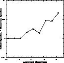
higher for fainter objects (see Fig. 2): note, however, that the
maximum fraction of galaxies
for which the spectra did not provide a useful z determination is
of them correspond to undeblended pairs (see
Sect. 2) for which the object coordinates fall in between the two components,
while most cases are due to not well connected fibers or to observations with
bad weather conditions. This kind of incompleteness is
higher for fainter objects (see Fig. 2): note, however, that the
maximum fraction of galaxies
for which the spectra did not provide a useful z determination is ![]() for the faintest galaxies of our survey (
for the faintest galaxies of our survey (![]() ).
).
We have verified that the magnitude distribution of not-observed objects
(![]() ) is consistent with being a random extraction from the total
sample. The main bias for such objects is introduced
by the impossibility of observing, in a given OPTOPUS exposure, two
objects closer than
) is consistent with being a random extraction from the total
sample. The main bias for such objects is introduced
by the impossibility of observing, in a given OPTOPUS exposure, two
objects closer than ![]() 25 arcsec. Although the MEFOS observations
and the repeated observations of the same fields have reduced somewhat
this bias, it is still significantly present in the data. This is
clearly seen in Fig. 3 which shows the observed distribution of
nearest neighbour distances (
25 arcsec. Although the MEFOS observations
and the repeated observations of the same fields have reduced somewhat
this bias, it is still significantly present in the data. This is
clearly seen in Fig. 3 which shows the observed distribution of
nearest neighbour distances (![]() ) for the entire photometric catalogue
(4487 objects; solid histogram) and for the 444 objects which
have not been observed spectroscopically (dashed histogram). The curves
superimposed on the two histograms show the expected distributions of
) for the entire photometric catalogue
(4487 objects; solid histogram) and for the 444 objects which
have not been observed spectroscopically (dashed histogram). The curves
superimposed on the two histograms show the expected distributions of
![]() on the basis of the measured angular correlation function. The
excess of not-observed objects which have a neighbour at a distance
smaller than 50 arcsec is 132
on the basis of the measured angular correlation function. The
excess of not-observed objects which have a neighbour at a distance
smaller than 50 arcsec is 132 ![]() 14 (183 objects in the data while 54 would
be expected); some, less significant excess (35
14 (183 objects in the data while 54 would
be expected); some, less significant excess (35 ![]() 11) is present also for
11) is present also for
![]() in the range 50-100 arcsec. Another way of characterizing the
same bias is through the ratio between the not-observed objects and the
total number of objects in the photometric catalogue as a function of
in the range 50-100 arcsec. Another way of characterizing the
same bias is through the ratio between the not-observed objects and the
total number of objects in the photometric catalogue as a function of
![]() . This ratio is 0.31, 0.13 0.10, 0.06 for
. This ratio is 0.31, 0.13 0.10, 0.06 for ![]() ,
,
![]() ,
, ![]() ,
, ![]() ,
respectively. Because of this bias, the spectroscopic catalogue can not
be used in a straightforward way for studying, for example, the statistics
of the number of close pairs or for analyzing the three dimensional correlation
function on very small scales.
,
respectively. Because of this bias, the spectroscopic catalogue can not
be used in a straightforward way for studying, for example, the statistics
of the number of close pairs or for analyzing the three dimensional correlation
function on very small scales.
 |
Figure 2:
Fraction of failed spectra over the total number of observed objects
as a function of magnitude. Note that, even in the faintest bin, this fraction
is always lower than |
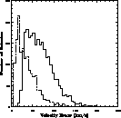
The errors on the velocities listed in Cols. (7) and (10) of Table 3 are
the formal errors given by the IRAF tasks XCSAO and EMSAO
for ![]() and
and ![]() , respectively. Their distributions are shown in
Fig. 4: the median error is 64 km/s for
, respectively. Their distributions are shown in
Fig. 4: the median error is 64 km/s for ![]() and 31 km/s for
and 31 km/s for ![]() .In order to have a better
estimate of the true errors, we have analyzed the differences in the
measured velocities (
.In order to have a better
estimate of the true errors, we have analyzed the differences in the
measured velocities (![]() ) of the galaxies which have been observed
more than once (156 galaxies with two measurements of
) of the galaxies which have been observed
more than once (156 galaxies with two measurements of ![]() and 64
galaxies with two measurements of
and 64
galaxies with two measurements of ![]() ).
For both these samples the histograms of
).
For both these samples the histograms of ![]() normalized to the formal
errors are significantly larger than expected if these formal errors were
correct estimates of the true errors.
By fitting these distributions with Gaussian
curves, the dispersions of the best fitting Gaussians are 1.53 and 2.10
for
normalized to the formal
errors are significantly larger than expected if these formal errors were
correct estimates of the true errors.
By fitting these distributions with Gaussian
curves, the dispersions of the best fitting Gaussians are 1.53 and 2.10
for ![]() and
and ![]() , respectively. This implies that, assuming that
the ratio between the true and the formal errors is a constant for all
measurements, the true errors can be estimated by multiplying the errors
given in Table 3 by these factors.
, respectively. This implies that, assuming that
the ratio between the true and the formal errors is a constant for all
measurements, the true errors can be estimated by multiplying the errors
given in Table 3 by these factors.
 |
Figure 4:
Distribution of the errors on the measured velocity, for both
|
The factor found for ![]() is in agreement with other values reported in
the literature from similar analyses: for instance, Bardelli et al. (1994)
found a factor 1.87 from a comparison of two sets of OPTOPUS observations
(45 galaxies) reduced with different packages (IRAF and MIDAS)
and by different authors; Malumuth et al. (1992), using multiple observations
of 42 galaxies reduced in the same way, found a factor 1.6.
is in agreement with other values reported in
the literature from similar analyses: for instance, Bardelli et al. (1994)
found a factor 1.87 from a comparison of two sets of OPTOPUS observations
(45 galaxies) reduced with different packages (IRAF and MIDAS)
and by different authors; Malumuth et al. (1992), using multiple observations
of 42 galaxies reduced in the same way, found a factor 1.6.
For about 750 galaxies we could measure the redshift both
from absorption and from emission lines. The distribution of the difference
(![]() ) is well fitted by a Gaussian
peaked at
) is well fitted by a Gaussian
peaked at ![]() km/s.
We have performed a number of tests, and we can exclude a zero-point
error. Also in the Las Campanas redshift survey a similar systematic difference
between the absorption and the emission velocities
has been found, and the authors have chosen to correct for it by using a
separate average template with large Balmer lines to fit emission line
galaxies (Shectman et al. 1996).
They suggest that the systematic effect is mainly due to the
blend between
km/s.
We have performed a number of tests, and we can exclude a zero-point
error. Also in the Las Campanas redshift survey a similar systematic difference
between the absorption and the emission velocities
has been found, and the authors have chosen to correct for it by using a
separate average template with large Balmer lines to fit emission line
galaxies (Shectman et al. 1996).
They suggest that the systematic effect is mainly due to the
blend between ![]() and
and ![]() lines.
On the other hand, we have decided to use in any case
the best-fitting template, for sake of homogeneity in the
redshift measures.
A more general discussion about this point will be found in Cappi et al.
(1998).
lines.
On the other hand, we have decided to use in any case
the best-fitting template, for sake of homogeneity in the
redshift measures.
A more general discussion about this point will be found in Cappi et al.
(1998).
Copyright The European Southern Observatory (ESO)