In Fig. 6 (click here) we have compared the X-ray source intensity (count rate, Table 2 (click here), Col. 5) from the RASS with the radio flux density from the 4.75 GHz LMC survey (Table 2 (click here), Col. 4). A similar comparison for the SMC is shown in Fig. 7 (click here) where we compared the source radio flux from 4.85 GHz survey (Table 3 (click here), Col. 4) with the X-ray source intensity (count rate, Table 3 (click here), Col. 5) from the ROSAT SMC PSPC surveys.
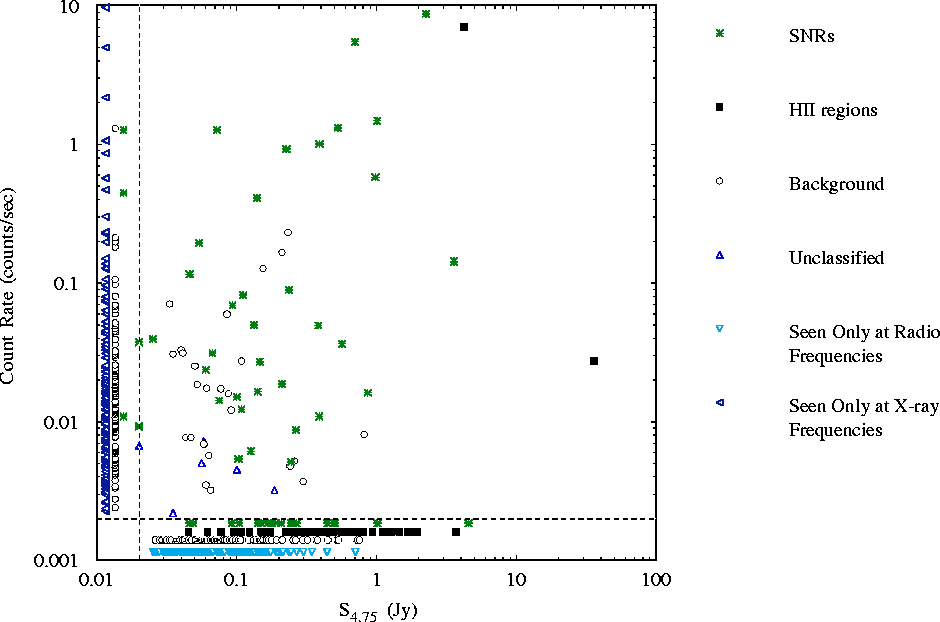
Figure 6: The distribution of X-ray count rate and radio flux
density at 4.75 GHz for different classes of sources in the
LMC. Asterisks represents SNRs; filled squares -
HII regions; open circles - background sources and open
triangles - unclassified sources. The dashed lines
represent the approximate threshold in radio and
X-ray surveys. Sources below the dashed lines
represent non-detections
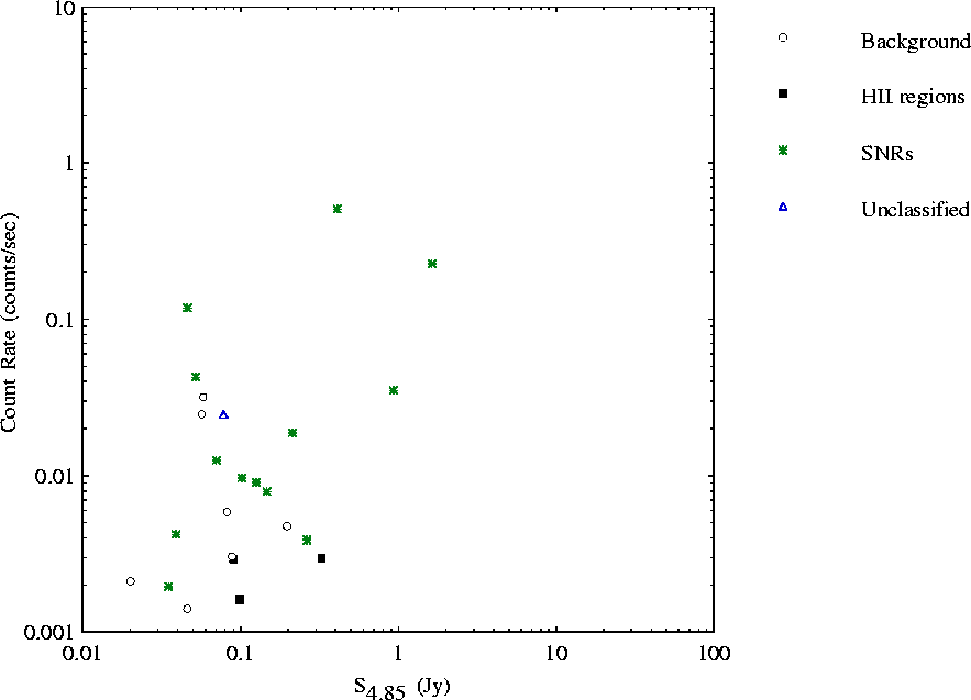
Figure 7: The distribution of X-ray count rate and radio
flux density at 4.85 GHz for different classes of
sources in the SMC. Asterisks represent SNRs; filled
squares - HII regions regions; open
circles - background sources and open
triangles - unclassified sources
Most of the radio sources in the field of the LMC (412 out of 483; 85%) fall below the sensitivity limit of the RASS survey (shown in Fig. 6 (click here) below 0.002 counts s-1) while most of the X-ray sources (254 out of 325; 78%) fall below the sensitivity limit of the radio survey (shown below 0.2 Jy). Many strong radio sources and strong X-ray sources have not been detected at X-ray and radio frequencies, respectively. For the SNRs embedded in HII regions, a small component of the radio flux will be caused by the HII regions but this will not significantly affect the radio-to-X-ray flux correlation.
There is very little correlation between radio and X-ray source intensities shown in Fig. 6. Of the sources observed at both radio and X-ray frequencies, the strongest at both frequencies tend to be SNRs. Breaking the sample of 483 radio sources into those above the X-ray threshold of 0.002 counts s-1 (71 sources) and those below (412 sources), the fraction of SNRs is 51% (36 out of 71) and 6% (26 out of 412), respectively.
Similar results can be seen in Fig. 7 (click here) where we compared the 27 sources in common towards the SMC. Seventeen of the SMC sources (SNRs and HII regions) are stronger emitters in both radio and X-ray frequencies than eight background and two unclassified sources.
We followed the classification of Chu & Kennicutt (1988b) for SNRs in
the LMC as Population I or Population II, to consider
the difference in X-ray and radio properties of the two types. In Fig. 8 (click here) the
X-ray Count Rate is plotted against the radio flux density (at 4.75 GHz)
for 32 SNRs distinguished by type. Nine SNRs are plotted as "unknown''
types. The interpolated 4.75 GHz flux densities were estimated from other
radio data for eight sources (flagged in Table 2 (click here), Col. 4) where no 4.75 GHz
flux densities are available. There is a large scatter in the ratio of
X-ray count rate to radio flux density. The ratio varies by three orders
of magnitude from 0.019 to 18 counts s-1 ![]() with median
0.38 counts s-1
with median
0.38 counts s-1 ![]() for the SNRs detected both at radio and X-ray.
If we consider SNRs detected at radio but not in X-ray, the range of
X-ray-to-radio ratio is even larger, with an upper limit as low
as
for the SNRs detected both at radio and X-ray.
If we consider SNRs detected at radio but not in X-ray, the range of
X-ray-to-radio ratio is even larger, with an upper limit as low
as ![]() counts s-1 Jy-1. However, there is a
tendency for SNRs which are strong in the radio to be also strong in X-rays.
counts s-1 Jy-1. However, there is a
tendency for SNRs which are strong in the radio to be also strong in X-rays.
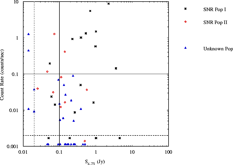
Figure 8: The distribution of X-ray count rate and radio flux
density at 4.75 GHz for different population of LMC SNRs.
Asterisks represent Population I SNRs; open
diamonds - Population II SNRs; and filled triangles
SNRs of unknown population. Population I SNRs tend to
be strong in both radio and X-ray surveys. The sample of sources
with both strong radio and X-ray intensities is dominated
by Population I SNRs
Figure 8 (click here) shows that young SNRs from Population I appear in the top right-hand corner with strong X-ray and radio intensities. Dividing this sample at arbitrary values of 0.1 Jy and 0.1 counts s-1, we note that the quadrant with strong radio and X-ray intensities is dominated by SNRs of Population I. Here 89% (8 out of 9) are Population I while in the other quadrants the fraction is 19% (6 out of 32) for the quadrant of strong radio and weak X-ray (including the sources below the X-ray threshold), 19% (3 out of 16) for weak radio, weak X-ray (including the sources below both thresholds) and 20% (1 out of 5) for weak radio, strong X-ray (including the sources below the radio threshold).
Population I SNRs are young and usually occur within large HII regions. This could be one reason for the occasional detection of X-ray emission from HII regions. Young Population II SNRs in the LMC are usually Balmer-dominated and occur in regions not interacting with other sources. They are, therefore, relatively weak X-ray and radio emitters. This could be a significant fact in SNR evolution; however, we can not rule out selection effects or a bias resulting from the small number of classified SNRs.