The elements of a model for echelle spectrographs are mirrors, lenses, gratings, prisms, grisms. Here we will focus solely on the geometric aspects, i.e. the 2D-dispersion relation. Luminosity aspects brought about by the interference terms, e.g. the echelle blaze function, line spread functions, as well as geometrical vignetting or reflectivity and transmissivity of materials will be the subject of subsequent communications. The notations of Schroeder (1987) are followed for the definitions of angles and orientations (right-hand Cartesian frame).
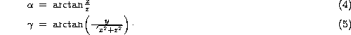
A ray incident on an optical surface co-planar with the xy-plane has
direction ![]() (see Fig. 1 (click here)) and projects onto the
axes as
(see Fig. 1 (click here)) and projects onto the
axes as

Conversely the angles ![]() are given by
are given by
![]()
Figure 1: Axes and angles notations
Since these angles are for incidences, their values are comprised in the
interval ![]() to
to ![]() . The orientation of the
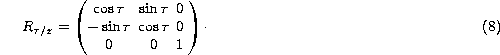
optical surface is described by the rotation angle
. The orientation of the
optical surface is described by the rotation angle ![]() about the
z axis. The angles
about the
z axis. The angles ![]() and
and ![]() denote rotations relative to x and y
respectively. Referential changes are performed by applying the rotations in
the following order:
denote rotations relative to x and y
respectively. Referential changes are performed by applying the rotations in
the following order:
![]()
and the transpose matrix provides the opposite change of the referential:
![]()
where each rotation matrix is of the form:
The direction of incident rays on an echelle grating
is defined by the two angles ![]() (Schroeder
1987). The general grating equation can be written as
(Schroeder
1987). The general grating equation can be written as
![]()
and
![]()
where m is the order number, ![]() the wavelength,
the wavelength, ![]() the
groove separation in unit of length, n and n' the refractive
indices before and after the grating,
the
groove separation in unit of length, n and n' the refractive
indices before and after the grating, ![]() and
and ![]() the
incidence angles, and
the
incidence angles, and ![]() and
and ![]() the direction of the
diffracted rays.
the direction of the
diffracted rays.
For a reflection grating n' = -n and therefore ![]() , hence
, hence
![]()
One can note that using the projection equations it is possible to
write the two grating Eqs. (9) and (10) as:
![]()
This formulation allows to introduce the grating in the model in the
form of a matrix. However, since no simple optical equation allows to
derive z this term will need to be derived from the normalization
relation:
![]()
The echelle relation of a spectrograph derives from the echelle grating
equation. For a constant ![]() and all rays
corresponding to a constant product
and all rays
corresponding to a constant product ![]() are diffracted in the
direction
are diffracted in the
direction ![]() . In a simplistic model one could expect that the
lines of constant value
. In a simplistic model one could expect that the
lines of constant value ![]() project as straight lines in the
detector planes and for a perfect alignment of the detector as, say,
columns on the detector. This assumption is however limited by aberrations
and rotation of the detector.
project as straight lines in the
detector planes and for a perfect alignment of the detector as, say,
columns on the detector. This assumption is however limited by aberrations
and rotation of the detector.
The cross-disperser is either a grating, a prism or a grism of low
spectral resolution. It displaces successive orders of the echelle grating
vertically with respect to each other. It is normally rotated by an angle
![]() so that the dispersion equations of the
cross-disperser needs to be applied after rotation to the referential of the
cross-disperser.
so that the dispersion equations of the
cross-disperser needs to be applied after rotation to the referential of the
cross-disperser. ![]() denotes the groove separation for
this grating.
denotes the groove separation for
this grating.
The refraction at a plane is given by Snell-Descartes law
![]()
The projection of an incident beam is given by Eq. (1 (click here))
and the angle ![]() with the z axis is:
with the z axis is:
![]()
One can also express this relation using the direction
cosine vector:
For n' = -n these are the equations for a mirror. This paper does not discuss grism based spectrographs although the above equations have been used to model such spectrographs. We indicate it here for the sake of completeness of the analytical framework. Grisms are represented by the association of a plane and a grating.
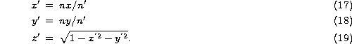
In the referential of the optical element the projections (x,y) on
the focal plane at focal distance F are given by
![]()
Equations (4) and (5) allow to derive directly the values of
![]() and
and ![]() from the coordinates of the unit
vector (x,y,z).
from the coordinates of the unit
vector (x,y,z).
Translation and rotation of the detector array are applied to the vector
point (x,y) by
![]()
This rotation can be applied as a rotation matrix before entering the camera lens. This step is performed after the lens projection in order to determine the analytical form of the dispersion relation in the absence of detector rotation.
In a complete optical train the above set of equations strictly apply only for on-axis rays and do not take into account field distortions, camera aberrations and wavelength dependencies of e.g. the focal lengths. In instruments like UVES (discussed below) these effects can account for discrepancies of several pixels at the detector.
Distortions are specific to the optical elements and layout, and are usually predictable and stable in time. As will be shown in Sect. 3 a model for a given instrument will typically match 99.5% using the physical description as developed above. For most applications it will not pay off to develop further the description by introducing off-axis optical equations. Instead the residuals can be corrected for by inserting at the proper location low order polynomial functions whose coefficients can for example be produced with the help of a ray tracing program.
In the following we will closely analyze the application of both, the exact (on axis) equations and a simplified analytical form respectively. Two notions of accuracy will be used. On the one hand the absolute accuracy of the model is limited by the optical effects not taken into account like e.g. aberrations and distortions. On the other hand the accuracy of the simplified analytical model will be limited by the numerical approximations performed to keep the analytical form simple (e.g. Taylor series expansions).