In most cases, even by looking at a reddened spectrum, one can roughly
assign the excitation level of the emitting nebula. The classification
scheme applied here is the one suggested by Aller (1956) with a
slight modification. A scale from 0 to 10 is used in the system. For low
excitation (classes ![]() 5), the [OII]
5), the [OII]![]() 3727/[OIII]
3727/[OIII]![]() 4959
ratio is used as a main indicator, while for the higher classes, the
ratio of HeII
4959
ratio is used as a main indicator, while for the higher classes, the
ratio of HeII ![]() 4686 to HeI
4686 to HeI ![]() 5876 is an imporant
criterion. In many cases, the ratio of lines originating from [ArIII],
[ArIV] and [ArV] have been taken into consideration
(see the discussion
by Ratag & Pottasch 1990). The limited sensitivity and
wavelength coverage in the spectra analyzed in this program do not allow us
to use the more sensitive indicators such as the ratio [NeV]
5876 is an imporant
criterion. In many cases, the ratio of lines originating from [ArIII],
[ArIV] and [ArV] have been taken into consideration
(see the discussion
by Ratag & Pottasch 1990). The limited sensitivity and
wavelength coverage in the spectra analyzed in this program do not allow us
to use the more sensitive indicators such as the ratio [NeV]![]() 3425/[NeIII]
3425/[NeIII]![]() 3868 in the nebulae with very
high excitation. The classification beyond class 7 should be thus considered
as uncertain by about 1 class.
3868 in the nebulae with very
high excitation. The classification beyond class 7 should be thus considered
as uncertain by about 1 class.
The most important parameters which contribute to determine the
excitation class of a nebula are the effective temperature of the
exciting star, the geometrical dilution factor, the optical depth in
the Lyman continuum, and the abundances. In order to eliminate the
dependence on the last factor, we should, in principle, avoid using a
ratio between lines originating from different elements, viz. the ratios
[OIII](![]() 4959 + 5007)/H
4959 + 5007)/H![]() , HeII
, HeII![]() 3868/H
3868/H![]() , in
determining the class as the abundances can vary by a large factor from
nebula to nebula. An example of a system which neglects the abundance
variational effect is the one proposed by Feast (1968), and
used by Webster (1988) in classifying the nebulae in her
sample.
, in
determining the class as the abundances can vary by a large factor from
nebula to nebula. An example of a system which neglects the abundance
variational effect is the one proposed by Feast (1968), and
used by Webster (1988) in classifying the nebulae in her
sample.
The excitation class distribution of the bulge PNe considered here is
shown in Fig. 2 (click here). The distribution has a peak around the classes 5
and 6. Comparisons are made with the bright nearby nebulae and the (smaller)
bulge sample studied by Webster (1988).
The former are taken from Aller & Czyzak (1983), Aller &
Keyes (1987), Pottasch (1984), Peimbert et al.
(1987b). The nearby nebulae seem to show an excess of high
excitation objects and lack of low excitation nebulae compared to the total
bulge sample. The bulge distribution is shifted toward the lower excitation
by about 1.5 to 2 classes with respect to the nearby sample. Some
possibilities can be put forward to explain this. The difference in the high
excitation range could be due to selection effect, as the PNe with high
central star temperatures tend to have a relatively larger size and lower
surface brightness, and thus are difficult to observe in the bulge
region. Although this could explain the high excitation excess, it is
certainly not able to explain the lack of objects in the opposite
extreme. The low excitation nebulae must be much easier to observe if
they are nearby. Another alternative is that the bulge PNe are ionized
by stars which have on average lower effective temperatures. Ratag et
al. (1990) examined this tendency and argued that it is independent
of the selection effect just mentioned above. They found the mean
![]() for the bulge PNe of about 45000 K, while for the
non-bulge sample, independent of size, the value is almost twice as
high. We conclude that the difference in the excitation class
distribution between the bulge sample and the nearby nebulae is real and
simply reflects the difference in their
for the bulge PNe of about 45000 K, while for the
non-bulge sample, independent of size, the value is almost twice as
high. We conclude that the difference in the excitation class
distribution between the bulge sample and the nearby nebulae is real and
simply reflects the difference in their ![]() distribution.
distribution.

Figure 2: The excitation class distribution of the bulge PNe
studied in this work (full thick) is compared with that of the nearby
nebulae (dashed) and that of the smaller bulge PN sample studied by
Webster (1988) (dashed-dotted). The last sample shows a
similarity to the total bulge sample. Both are shifted by approximately 1.5
to 2 classes toward lower excitation range with respect to the nearby
nebulae. This is probably due to the difference in their cental star
effective temperature distribution
The second comparison is made with Webster's sample. Using the Feast (1968) system she found that the excitation class distribution is fairly uniform over the whole excitation range. As pointed out previously, the Feast system is affected by the abundance. We have reclassified the objects according to Aller's scheme and display the distribution in Fig. 2 (click here) as a dashed-dotted histogram. We include also a few objects, mainly the low excitation one, which do not have the important lines necessary for the plasma diagnostics and therefore have been excluded from the total bulge sample. The resulting distribution clearly shows a non-unformity, and is very similar to the total sample, having a peak at about classes 5 and 6.
The plasma diagnostics were done in ![]() diagrams where we
plotted the dependence on temperature and density of the available
forbidden line intensity ratios. In all computations we made use of the
atomic parameters compiled by Mendoza (1983) supplemented with
new data recommended by Clegg (1989). We calculated the
populations of up to fifteen levels of each ion in order to obtain the
theoretical intensity ratios.
diagrams where we
plotted the dependence on temperature and density of the available
forbidden line intensity ratios. In all computations we made use of the
atomic parameters compiled by Mendoza (1983) supplemented with
new data recommended by Clegg (1989). We calculated the
populations of up to fifteen levels of each ion in order to obtain the
theoretical intensity ratios.
The electron temperature ![]() indicators in our spectra are the
ratios of [OIII](
indicators in our spectra are the
ratios of [OIII](![]() 4959+
4959+![]() 5007)/
5007)/![]() 4363 and
[NII](
4363 and
[NII](![]() 6548+
6548+![]() 6583)/
6583)/![]() 5755.
On several occasions the
ratios [OII]
5755.
On several occasions the
ratios [OII]![]() 7325/
7325/![]() 3727 and
[SII](
3727 and
[SII](![]() 4068+
4068+![]() 4076)/ (
4076)/ (![]() 6717+
6717+![]() 6731) provide
secondary information. The uncertainties in
6731) provide
secondary information. The uncertainties in ![]() determinations are mainly due to the weakness of
determinations are mainly due to the weakness of ![]() 4363 and
4363 and
![]() 5755 lines. For a relatively faint
5755 lines. For a relatively faint ![]() 4363 line, an
uncertainty in intensity of about 25% should be allowed. This leads to a
resulting
4363 line, an
uncertainty in intensity of about 25% should be allowed. This leads to a
resulting ![]() with an imprecision of about 10%. A
relatively strong
with an imprecision of about 10%. A
relatively strong ![]() 4363 line, with an accuracy of better than
15%, would lead to a
4363 line, with an accuracy of better than
15%, would lead to a ![]() with uncertainty of about 5%.
The [NII]
with uncertainty of about 5%.
The [NII]![]() 5755 lines are generally less precise, and we
suggest that the accuracy in the resulting
5755 lines are generally less precise, and we
suggest that the accuracy in the resulting ![]() [NII] is
between 5% to 15% worse than that related to the
[NII] is
between 5% to 15% worse than that related to the
![]() [OIII].
[OIII].
The main density indicator used in this program is the [SII] doublet at
about 6725 Å. Reasonably good atomic data for [ArIV] are now
available thanks to the computation by Zeippen et al. (1987).
The line intensity ratio [ArIV]![]() 4711/
4711/![]() 4740 can be
used as a reliable diagnostic for electron density. The use of this line
ratio usually involves a self-consistent iterative procedure in order to
subtract the possible contribution of HeI and [NeIV] emission at
4740 can be
used as a reliable diagnostic for electron density. The use of this line
ratio usually involves a self-consistent iterative procedure in order to
subtract the possible contribution of HeI and [NeIV] emission at
![]() 4711. The HeI can be easily predicted from the
HeI
4711. The HeI can be easily predicted from the
HeI ![]() 5876, while the subtraction of the [NeIV] lines requires us to examine
the ionization structure to estimate the ratio of N(Ne3+) to
N(Ne++). The latter is usually well represented in the spectra at
5876, while the subtraction of the [NeIV] lines requires us to examine
the ionization structure to estimate the ratio of N(Ne3+) to
N(Ne++). The latter is usually well represented in the spectra at
![]() 3868 and
3868 and ![]() 3968 (blended with
3968 (blended with ![]() ). Having
subtracted the contributions of HeI and [NeIV] lines we
redetermined the
). Having
subtracted the contributions of HeI and [NeIV] lines we
redetermined the
![]() with the corrected [ArIV]
with the corrected [ArIV]![]() 4711, and eventually
remodelled the nebula. The procedure was repeated (for 4 to 5
iterations)
until a satisfactory
consistency was achieved. In a small number of cases, the density sensitive
doublets of [CIII] are available and have also been applied. The
advantage of using [ArIV] and [CIII] line ratios is that for
the medium
to high excitation and for the high density (
4711, and eventually
remodelled the nebula. The procedure was repeated (for 4 to 5
iterations)
until a satisfactory
consistency was achieved. In a small number of cases, the density sensitive
doublets of [CIII] are available and have also been applied. The
advantage of using [ArIV] and [CIII] line ratios is that for
the medium
to high excitation and for the high density (![]() 5000 cm-3) nebulae the derived electron density is more
representative for the whole nebula than that derived from the [SII]
doublet. Unfortunately, the corresponding lines are usually much weaker
than those coming from the
5000 cm-3) nebulae the derived electron density is more
representative for the whole nebula than that derived from the [SII]
doublet. Unfortunately, the corresponding lines are usually much weaker
than those coming from the ![]() ions.
ions.
Since the distance to the nebulae are reasonably well known (d = 7.7
kpc; Reid 1989) with an uncertainty of probably less than 20%,
and because the sizes, the radio continuum flux densities and/or the
H![]() flux measurements are already available for almost all the
nebulae, it is possible to determing the
flux measurements are already available for almost all the
nebulae, it is possible to determing the ![]() (rms) (
(rms) (![]() ;
; ![]() is the
filling factor defined as the ratio between the filled and the total volume)
with reasonably good accuracy. To calculate the
is the
filling factor defined as the ratio between the filled and the total volume)
with reasonably good accuracy. To calculate the ![]() (rms),
the equation
(rms),
the equation
![]()
(Spitzer 1978) was used. Here ![]() is expressed in
mJy,
is expressed in
mJy, ![]() in K, d in kpc, and
in K, d in kpc, and ![]() , the angular radius of
the source, in arcsec, and
, the angular radius of
the source, in arcsec, and ![]() , where x =
N(He+/N(H+) and y = N(He)/N(H).
, where x =
N(He+/N(H+) and y = N(He)/N(H).
The electron densities derived from the [SII] lines are plotted against
the ![]() (rms) in Fig. 3 (click here). In this figure we
distinguish the small size objects (with a diameter
(rms) in Fig. 3 (click here). In this figure we
distinguish the small size objects (with a diameter ![]() 3 arcsecs) from
the larger ones. Some important remarks can be made from the figure. The
spread is usually interpreted as due to the non-uniformity in the densities.
Since for most of bulge nebulae the observed lines come from the whole
object rather than from a small region, the filling factor
3 arcsecs) from
the larger ones. Some important remarks can be made from the figure. The
spread is usually interpreted as due to the non-uniformity in the densities.
Since for most of bulge nebulae the observed lines come from the whole
object rather than from a small region, the filling factor ![]() can be
estimated such that
can be
estimated such that ![]() (FL)
(FL)![]() =
=
![]() (rms). For the nebulae lying below the line
corresponding to
(rms). For the nebulae lying below the line
corresponding to ![]() = 1.0, this brings a special problem
since the derived
= 1.0, this brings a special problem
since the derived ![]() will be larger than unity. This is
generally not caused by the error in the adopted distance or in the size
determination. Even if the distances are wrong by about 2 kpc, the
discrepancies from the line with
will be larger than unity. This is
generally not caused by the error in the adopted distance or in the size
determination. Even if the distances are wrong by about 2 kpc, the
discrepancies from the line with ![]() = 1.0 are still large.
Allowing
an error of about 25% in the size determinations can shift the
points by only about 0.145 dex to the left. The deviations are still
present.
= 1.0 are still large.
Allowing
an error of about 25% in the size determinations can shift the
points by only about 0.145 dex to the left. The deviations are still
present.
Another further point is of interest regarding Fig. 3 (click here). The problem
we just mentioned is almost always met when the ![]() (rms) is
higher than about 5000 cm-3, and when the angular diameter is less
than about 3 arcsecs. A higher density, and thus a higher optical depth,
will result in a larger drop in the specific intensity J(v) as we
proceed away from the star. If the distance from the ionizing star to
the nebula is still relatively small, the dilution factor for the inner
region can differ by a large factor from that for the outer region. As
the nebula evolves, expanding with an assumed uniform velocity, this
difference will become smaller. Consequently, in the case of small,
dense and especially medium to high excitation nebulae, the electron
density obtained from the [SII] lines is likely to represent the region
near the periphery where the ionization has dropped by a large factor
and thus having lower
(rms) is
higher than about 5000 cm-3, and when the angular diameter is less
than about 3 arcsecs. A higher density, and thus a higher optical depth,
will result in a larger drop in the specific intensity J(v) as we
proceed away from the star. If the distance from the ionizing star to
the nebula is still relatively small, the dilution factor for the inner
region can differ by a large factor from that for the outer region. As
the nebula evolves, expanding with an assumed uniform velocity, this
difference will become smaller. Consequently, in the case of small,
dense and especially medium to high excitation nebulae, the electron
density obtained from the [SII] lines is likely to represent the region
near the periphery where the ionization has dropped by a large factor
and thus having lower ![]() . The best photoionization models
of these nebulae show that this is indeed the case. Accordingly, for
such nebulae we have always adopted the
. The best photoionization models
of these nebulae show that this is indeed the case. Accordingly, for
such nebulae we have always adopted the ![]() (rms) as the
relevant density to derive the atomic hydrogen number density
(rms) as the
relevant density to derive the atomic hydrogen number density ![]() .
For this particular reason we have reanalysed two objects, PK 357+2.4
and PK 356-4.1, from Aller & Keyes (1987) sample.
In their analysis, electron densities of respectively, 7500 cm-3
and 4000 cm-3 were adopted, while the radio continuum measurements
(Gathier et al. 1983; Zijlstra et al. 1989)
indicate that values much higher than 104 cm-3 should be used. In
the case of PK 356-4.1 the newly derived abundances differ only by about
15% to 25% from the previous results but for PK 357+2.4 these differences
are, on average, 40% which stress the importance of the problem.
.
For this particular reason we have reanalysed two objects, PK 357+2.4
and PK 356-4.1, from Aller & Keyes (1987) sample.
In their analysis, electron densities of respectively, 7500 cm-3
and 4000 cm-3 were adopted, while the radio continuum measurements
(Gathier et al. 1983; Zijlstra et al. 1989)
indicate that values much higher than 104 cm-3 should be used. In
the case of PK 356-4.1 the newly derived abundances differ only by about
15% to 25% from the previous results but for PK 357+2.4 these differences
are, on average, 40% which stress the importance of the problem.
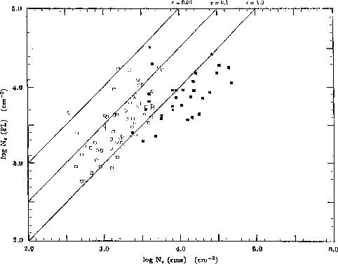
Figure 3: The electron density derived from the radio continuum
measurements, ![]() (rms) =
(rms) = ![]() (
(![]() is the filling factor) plotted against the density obtained
from the forbidden line ratio of [SII]. The three straight lines are the
expectations of a simple model with filling factor
is the filling factor) plotted against the density obtained
from the forbidden line ratio of [SII]. The three straight lines are the
expectations of a simple model with filling factor ![]() = 0.01,
= 0.01,
![]() = 0.1, and
= 0.1, and ![]() = 1.0 (uniform). The nebulae with a
diameter equal to or less than 3 arcsecs are represented by the filled
symbol
= 1.0 (uniform). The nebulae with a
diameter equal to or less than 3 arcsecs are represented by the filled
symbol
Tables 2a and 2b list some important parameters of the objects
investigated in the present program. Table 2a is for the newly observed
objects discussed in Sect. 2.1, and Table 2b is for those of which the
spectra are taken from literature (Sect. 2.2). Both tables are arranged
as follows. In Cols. 1 and 2, we give the PK-designation and the
usual name of the nebula. Column 3 lists the excitation class as
discussed in Sect. 3.1. The radio continuum flux density at 6-cm is
given in Col. 4 in units of mJy. They are mostly from the works of
Gathier et al. (1983) and Zijlstra et al. (1989).
The H![]() flux (in units of erg cm-2 s-1) is tabulated in
Col. 5 in logarithmic form. The next Col. 6 gives the angular diameter of
the nebula in arcsecs, measured mostly by the VLA by Gathier et al. and
Zijlstra et al. In a few cases the optical diameters were adopted. The
E(B-V)s derived by using the Balmer decrement method and by comparing the
expected H
flux (in units of erg cm-2 s-1) is tabulated in
Col. 5 in logarithmic form. The next Col. 6 gives the angular diameter of
the nebula in arcsecs, measured mostly by the VLA by Gathier et al. and
Zijlstra et al. In a few cases the optical diameters were adopted. The
E(B-V)s derived by using the Balmer decrement method and by comparing the
expected H![]() flux, based on radio continuum measurements, with that
optically observed are given respectively in Cols. 7 and 8. The
electron temperature obtained from the plasma diagnostics are listed in
Cols. 9 (OIII), 10 (NII) and 11. The
flux, based on radio continuum measurements, with that
optically observed are given respectively in Cols. 7 and 8. The
electron temperature obtained from the plasma diagnostics are listed in
Cols. 9 (OIII), 10 (NII) and 11. The ![]() presented in Col. 11 is the average expected for the whole nebula. In
the next Col. (12), we list the electron density
presented in Col. 11 is the average expected for the whole nebula. In
the next Col. (12), we list the electron density ![]() as
derived from the forbidden line intensity ratios ([SII], [ArIV] and [ClIII]).
These various line ratios allow a density diagnostic up to about 20000
cm-3. Column 13 gives
as
derived from the forbidden line intensity ratios ([SII], [ArIV] and [ClIII]).
These various line ratios allow a density diagnostic up to about 20000
cm-3. Column 13 gives ![]() , the radial velocity in km s-1
referred to the local standard of rest as adopted from the catalog of
Schneider et al. (1983). For Table 2a there is an additional
column, i.e. Col. 14, which gives the ratio of the observed continuum flux
at
, the radial velocity in km s-1
referred to the local standard of rest as adopted from the catalog of
Schneider et al. (1983). For Table 2a there is an additional
column, i.e. Col. 14, which gives the ratio of the observed continuum flux
at ![]() 5325 Å to H
5325 Å to H![]() flux density, appropriate for the
derivation of the central star effective temperature. The total infrared
flux
flux density, appropriate for the
derivation of the central star effective temperature. The total infrared
flux ![]() , based on the IRAS measurements and derived by
integrating between
, based on the IRAS measurements and derived by
integrating between ![]() and
and ![]() are shown in the
15th column of Table 2a and 14th of Table 2b. In Col. 16 of Table 2a and
Col. 15 of Table 2b, we list the infrared excess (IRE) computed by
using equation (VIII-11) of Pottasch (1984), taking into
account the dependence on density and in a small number of cases, on the
optical depth at 6-cm. The letter symbols given in the last column are
references listed at the end of the tables.
are shown in the
15th column of Table 2a and 14th of Table 2b. In Col. 16 of Table 2a and
Col. 15 of Table 2b, we list the infrared excess (IRE) computed by
using equation (VIII-11) of Pottasch (1984), taking into
account the dependence on density and in a small number of cases, on the
optical depth at 6-cm. The letter symbols given in the last column are
references listed at the end of the tables.