Because of the large velocity range covered by the Galactic Center
emission, position switching was chosen as the observing mode. This
observing mode produces flat baselines only if the atmospheric
conditions for the ON and OFF positions are very similar,
i.e., if their positions on the sky are not very different and the
weather conditions are stable. Unfortunately, the Galactic Center
region shows extremely extended emission, so that nearby emission-free
positions are difficult to find, in particular with a 9![]() telescope beam. Therefore, the OFF positions often had to be
several degrees distant from the ON position.
telescope beam. Therefore, the OFF positions often had to be
several degrees distant from the ON position.
Flat baselines result if the difference power, DP, between the OFF
and the ON positions is minimized. To achieve this, the following
scheme is used (weighted-OFFs mode): The telescope control program
picks two OFF positions from a given list of emission-free positions,
one at higher and one at lower elevation than the ON position based
on a weight assigned to each OFF position for its horizontal distance
on the sky from the ON position and for the predicted DP, from an
atmospheric model, due to the distance in elevation. This elevation
weighting takes into account the increment of air masses with decreasing
elevation as well as the fact that, in worse weather conditions, there must
be a smaller distance in elevation of appropriate OFF positions to
the ON position. The weighting formula is as follows:
![]()
where the second term is the predicted difference power, DP, squared. The
term, ![]() , is the normalization factor for the distance in
azimuth which indicates what distance in azimuth in degrees is weighted
equally to a DP of 1 K.
, is the normalization factor for the distance in
azimuth which indicates what distance in azimuth in degrees is weighted
equally to a DP of 1 K.
The choice of this normalization factor had to be empirical because
distance in azimuth and difference power are very different quantities. In
principle, azimuth changes should not matter, since these do not produce
any systematic change in power. But atmospheric variations from position to
position do occur. Also, as one switches further in azimuth, the time
between ON and OFF increases, so that there are gain variations
which increase with time. At the 1.2m SMWT, 0.65 was determined to be the
best choice for ![]() .
.
After weighting all the OFF positions for their current azimuth and elevation, the program chooses the best OFF position (lowest weight) as the first OFF (subscan A) and the best OFF position on the opposite side in elevation of the ON position as second OFF (subscan B). If the first OFF has an extremely low weighting value (nearly the same elevation as the ON position) only this OFF may be used for the complete scan. See Dame (1992) for further details on the weighted-OFFs mode.
The integration of the two subscans was done in 30-second-cycles, the first half of which was spent on the OFF position. Note that the integration time of the scans is the sum of the integration time on source and on the OFF positions.
Every subscan is started with a calibration lasting 5 seconds. The
calibration procedure follows the standard chopper wheel method first
described by Penzias & Burrus (1973) and applied at many
other millimeter telescopes. Following this method, the temperature in
channel i is calculated from:
![]()
where Vi are the voltage outputs of each channel during the scan
integration on source (![]() ), on the OFF position
(
), on the OFF position
(![]() ), during the calibration on the chopper wheel
(
), during the calibration on the chopper wheel
(![]() ), and on the sky (
), and on the sky (![]() ), see
Ulich & Haas (1976), Downes (1989) for
details.
), see
Ulich & Haas (1976), Downes (1989) for
details. ![]() is the elevation and weather dependent
conversion factor from the measured voltage to the antenna temperature
. This factor corrects for atmospheric attenuation in the signal
and image sideband, and implicitly for resistive losses and rearward
spillover and scattering (see Eq. (4) in Downes 1989 and
Eq. (17) in Ulich & Haas 1976).
is the elevation and weather dependent
conversion factor from the measured voltage to the antenna temperature
. This factor corrects for atmospheric attenuation in the signal
and image sideband, and implicitly for resistive losses and rearward
spillover and scattering (see Eq. (4) in Downes 1989 and
Eq. (17) in Ulich & Haas 1976).
| |
C | |
|
| 0.2054 | 0.0380 |
|
| 0.0971 | 0.0650 |
|
| 255.0 K | 255.0 K |
|
| 254.0 K | 254.0 K |
Generally, the calibration conversion factor, ![]() , is
determined by carrying out an antenna tip, a procedure in which
, is
determined by carrying out an antenna tip, a procedure in which
![]() is measured as a function of air mass using a
two-layer atmospheric model, consisting of a time-constant upper layer of
O2 and a variable lower layer of H2O, as described in
Kutner (1978). The values for the opacity and temperature of
the oxygen "layer'' as used for the Cerro Tololo (altitude 2215 m) are
given in Table 3 (click here). The antenna tip has to be repeated
periodically; every six hours was found to be adequate. The zenith opacity
of water vapour was typically
is measured as a function of air mass using a
two-layer atmospheric model, consisting of a time-constant upper layer of
O2 and a variable lower layer of H2O, as described in
Kutner (1978). The values for the opacity and temperature of
the oxygen "layer'' as used for the Cerro Tololo (altitude 2215 m) are
given in Table 3 (click here). The antenna tip has to be repeated
periodically; every six hours was found to be adequate. The zenith opacity
of water vapour was typically ![]() . A more detailed description of
this calibration method is given in Appendix A of Cohen et
al. (1986).
. A more detailed description of
this calibration method is given in Appendix A of Cohen et
al. (1986).
Because of the possibility of confusion caused by different notations found in the literature, we give a full account of the relevant relations.
The antenna temperature is the natural result of chopper-wheel
calibration. However, is not appropriate for telescope and line
independent comparisons because it is not corrected for all telescope
losses (see, e.g., Downes 1989). is the brightness
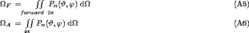
temperature of an equivalent source which fills the entire ![]() steradians
of the forward beam pattern; it can be thought of as a "forward-beam
brightness temperature''. Therefore, still contains the forward
beam pattern as a telescope dependent parameter. Besides the main beam
(MB), this consists of (1) the spillover of feed power around the
secondary, (2) the scattering from the aperture blockage caused by the
secondary mirror and its support structure, and (3) the diffraction
sidelobes through the finite aperture of the main mirror
(Cohen et al. 1986). The appropriate parameter for
comparison is the "main-beam brightness temperature'', , that is the
brightness temperature of a source which just fills the main beam.
is a property of the source itself; provided the source is resolved,
different radio telescopes will have the same value.
steradians
of the forward beam pattern; it can be thought of as a "forward-beam
brightness temperature''. Therefore, still contains the forward
beam pattern as a telescope dependent parameter. Besides the main beam
(MB), this consists of (1) the spillover of feed power around the
secondary, (2) the scattering from the aperture blockage caused by the
secondary mirror and its support structure, and (3) the diffraction
sidelobes through the finite aperture of the main mirror
(Cohen et al. 1986). The appropriate parameter for
comparison is the "main-beam brightness temperature'', , that is the
brightness temperature of a source which just fills the main beam.
is a property of the source itself; provided the source is resolved,
different radio telescopes will have the same value.
the forward efficiency, , is defined as the factor which scales
, the antenna temperature of an equivalent resistor outside the
atmosphere (thus, the antenna temperature corrected for atmospheric
losses), to :
![]()
Following the notation of Kraus (1986), the forward efficiency
is:
![]()
where k0 is the resistive loss factor of the telescope, ![]() the
forward-beam solid angle,
the
forward-beam solid angle, ![]() the antenna-beam solid angle. The
two latter are defined as follows:
the antenna-beam solid angle. The
two latter are defined as follows:
where ![]() is the antenna power pattern normalized to
its maximum value as a function of angle. Thus, a beam solid angle is the
angle inside of which a fictitious antenna must have a power pattern equal
to the maximum value of the antenna in use and outside which an antenna
power pattern equal to zero to receive the same complete power as the
antenna in use. Hence, the ratio
is the antenna power pattern normalized to
its maximum value as a function of angle. Thus, a beam solid angle is the
angle inside of which a fictitious antenna must have a power pattern equal
to the maximum value of the antenna in use and outside which an antenna
power pattern equal to zero to receive the same complete power as the
antenna in use. Hence, the ratio ![]() is the
fraction of the total power which enters the forward beam.
is the
fraction of the total power which enters the forward beam.
Similar to the definition of , the effective beam efficiency, ,
is defined as the factor which scales to
(Downes 1989):
![]()
Following again the notation of Kraus (1986), the effective
beam efficiency is:
![]()
where ![]() is the main-beam solid angle given by the equation:
is the main-beam solid angle given by the equation:
![]()
Therefore, the ratio ![]() is the fraction of the
total power which enters the main beam.
is the fraction of the
total power which enters the main beam.
Summarizing, to scale to one has to multiply
by the ratio of to (Eqs. (A3 (click here)) and
(A7 (click here))):
![]()
With the Eqs. (A4 (click here)) and (A8 (click here)) the ratio of to
can be written as:
![]()
In other words, this ratio indicates the fraction of the forward power
which enters the main beam.
which was used previously for the calibration of the data for the 1.2m
NMWT and SMWT, , the antenna temperature of an equivalent resistor
outside the atmosphere, is related to ![]() , the true source
Rayleigh-Jeans brightness temperature (called in the notation of
Downes 1989), by:
, the true source
Rayleigh-Jeans brightness temperature (called in the notation of
Downes 1989), by:
![]()
where ![]() is the resistive loss factor of the telescope, called k0
by Kraus (1986), defined in terms of the maximum antenna gain
G as:
is the resistive loss factor of the telescope, called k0
by Kraus (1986), defined in terms of the maximum antenna gain
G as:
![]()
where ![]() is the solid angle subtended by the response of the
source in the beam pattern, given by:
is the solid angle subtended by the response of the
source in the beam pattern, given by:
![]()
To separate the convolution of the source structure with the antenna beam
pattern, Kutner & Ulich define the radiation temperature
![]() as the source intensity which is corrected for all effects
except the actual coupling of the antenna diffraction pattern to the source
brightness distribution. Thus,
as the source intensity which is corrected for all effects
except the actual coupling of the antenna diffraction pattern to the source
brightness distribution. Thus, ![]() is related to
is related to ![]() by:
by:
![]()
where ![]() is the efficiency with which the antenna couples to the
source. This is given by:
is the efficiency with which the antenna couples to the
source. This is given by:
![]()
with:
![]()
Thus, ![]() is the diffraction-beam solid angle, and the diffraction
area over which it is integrated in this equation is the area which covers
the normal diffraction pattern of the antenna. Typically, this area will
encompass a region within a few degrees of the telescope axis.
is the diffraction-beam solid angle, and the diffraction
area over which it is integrated in this equation is the area which covers
the normal diffraction pattern of the antenna. Typically, this area will
encompass a region within a few degrees of the telescope axis.
With this, is related to ![]() by:
by:
![]()
Because the forward spillover and scattering arises from the sky, at
sky temperature, and the rearward spillover and scattering from the
ground, at ambient temperature, Kutner & Ulich divided the
spillover and scattering efficiency ![]() into the
product of the forward (
into the
product of the forward (![]() ) and the rearward (
) and the rearward (![]() ) part, given by:
) part, given by:

Defining the telescope efficiency ![]() and the extended source
efficiency
and the extended source
efficiency ![]() as:
as:
![]()
Kutner & Ulich obtained:
![]()
Thus, ![]() is related to by:
is related to by:
![]()
As Kutner & Ulich have shown, ![]() can be fitted by
an antenna tipping procedure because the observed antenna temperature of the
sky,
can be fitted by
an antenna tipping procedure because the observed antenna temperature of the
sky, ![]() , is then given by:
, is then given by:
![]()
Because an antenna tipping was regularly done at the 1.2m SMWT (and NMWT)
during observations ![]() was always monitored. Averaged over the
complete observing time, it was 0.881
was always monitored. Averaged over the
complete observing time, it was 0.881 ![]() 0.023, thus, very stable.
0.023, thus, very stable.
Comparing the notation of Kutner & Ulich (1981) with the
notation of Downes (1989) it becomes clear that ![]() is (compare Eqs. (A20 (click here)), (A21 (click here)), and (A23 (click here))
with Eqs. (A3 (click here)) and (A4 (click here))) but that
is (compare Eqs. (A20 (click here)), (A21 (click here)), and (A23 (click here))
with Eqs. (A3 (click here)) and (A4 (click here))) but that ![]() is
not (compare Eqs. (A19 (click here)), (A22 (click here)), and
(A24 (click here)) with Eqs. (A7 (click here)) and (A8 (click here))) because
is
not (compare Eqs. (A19 (click here)), (A22 (click here)), and
(A24 (click here)) with Eqs. (A7 (click here)) and (A8 (click here))) because ![]() is not equal to
is not equal to ![]() . However, as Downes
(1989) pointed out,
. However, as Downes
(1989) pointed out, ![]() is not a telescope constant,
but is a variable which must be evaluated as a function of the diameter of
the source to be observed. Thus,
is not a telescope constant,
but is a variable which must be evaluated as a function of the diameter of
the source to be observed. Thus, ![]() is not the appropriate
parameter for comparison purposes because this temperature still contains
the diffraction sidelobes through the finite aperture of the main mirror as
a telescope specific contribution. Therefore, observers who use the
notation of Kutner & Ulich (1981) are advised to choose
is not the appropriate
parameter for comparison purposes because this temperature still contains
the diffraction sidelobes through the finite aperture of the main mirror as
a telescope specific contribution. Therefore, observers who use the
notation of Kutner & Ulich (1981) are advised to choose
![]() as
as ![]() so that
so that ![]() becomes .
becomes .
the calibration is described in detail by Cohen et al. (1986)
for the NMWT and Bronfman et al. (1988) for the SMWT. To
derive intensities which are as independent as possible of the parameters
of the telescope, they both defined their "Mini''-![]() -- which they
called the main beam efficiency -- as the fraction of the forward power
that enters the main beam. It is the factor has to be divided by
to yield
-- which they
called the main beam efficiency -- as the fraction of the forward power
that enters the main beam. It is the factor has to be divided by
to yield ![]() , which they define as the physical temperature of a
black body that just fills the main beam. As Cohen et al.
(1986) pointed out, this
, which they define as the physical temperature of a
black body that just fills the main beam. As Cohen et al.
(1986) pointed out, this ![]() differs from
differs from ![]() as
defined by Kutner & Ulich (1981). It is defined in exactly
the same way as the main-beam brightness temperature, . Thus, results
obtained with the 1.2m Telescopes have long been in even though
this was not described as such, and the "Mini''-
as
defined by Kutner & Ulich (1981). It is defined in exactly
the same way as the main-beam brightness temperature, . Thus, results
obtained with the 1.2m Telescopes have long been in even though
this was not described as such, and the "Mini''-![]() , which is strictly
speaking the main-beam-to-forward-beam efficiency,
, which is strictly
speaking the main-beam-to-forward-beam efficiency, ![]() , is
given by:
, is
given by:
![]()
This ![]() was determined for the NMWT by Cohen et
al. (1986) and for the SMWT by Bronfman (1986) using
the theoretical radiation pattern of the feed horn, scalar diffraction
theory, and the measured antenna pattern. The result was checked
observationally and is the same for both telescopes:
was determined for the NMWT by Cohen et
al. (1986) and for the SMWT by Bronfman (1986) using
the theoretical radiation pattern of the feed horn, scalar diffraction
theory, and the measured antenna pattern. The result was checked
observationally and is the same for both telescopes:
![]()
When one applies all these corrections, one obtains the final calibration
of :

The coordinate system of the telescope was established with roughly
40 stars, sighted through a 3 cm optical telescope mounted on the
primary and coaligned with the radio axis because no point source can
be detected with a small telescope at millimeter wavelengths in short
integration times (Cohen 1977). This was done twice a year.
To check if a realignment of the telescope coordinate system is required,
every few days the pointing was checked in the radio by scanning through the
limbs of the Sun to determine its center to within 10![]() (Cohen et al. 1986; Grabelsky et al. 1987).
(Cohen et al. 1986; Grabelsky et al. 1987).
During the observations, the pointing accuracy was ensured by
monitoring the tracking of the telescope constantly. If the tracking
error exceeded the limit of 1![]() the integration was
interrupted. Therefore, the pointing of the 1.2m SMWT was always
better than 1
the integration was
interrupted. Therefore, the pointing of the 1.2m SMWT was always
better than 1![]() 0 (0.11 beamwidths at the
0 (0.11 beamwidths at the ![]() line frequency).
line frequency).