Inverse problems are very frequent in modern astronomy, as in many other
scientific and technical disciplines. They occur if unknown parameters of
an object or a phenomenon are related to observed data and if one wants to
estimate these parameters from the observed quantities, which, of course, can
be additionally distorted by a stochastic process like noise. Such problems
belong to the class of ill-posed problems for which the uniqueness of the
solution cannot be established and the solutions are oversensitive to the
input data perturbations (Hadamard 1923; Tikhonov & Arsenine 1977). The
discrete and linear version of the inverse problem (most frequently considered
in astronomy) has the form:
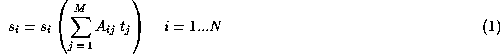
where ![]() are unknown, searched parameters,
are unknown, searched parameters, ![]() describe the transformation and
describe the transformation and
![]() represent observed data, which are random variables. They are in general any
statistics of one's choice (e.g. Poissonian in the case of astronomical images)
and of expectation values given by the bracketed term.
represent observed data, which are random variables. They are in general any
statistics of one's choice (e.g. Poissonian in the case of astronomical images)
and of expectation values given by the bracketed term.
Such inverse problems occur in astronomy in numerous cases, including,
e.g. mapping of emission line regions of AGN's (Mannucci et al. 1992), mapping
of accretion discs in binary systems (Horne 1985; Baptista & Steiner 1991),
surface imaging of stars (Piskunov & Rice 1993), mapping of active regions in
cometary nuclei (Waniak 1994). If the observed quantities and searched
parameters belong to the same data space and N is equal to M the inverse problem
becomes an image restoration.
A straightforward solution of Eq. (1) via matrix inversion (assuming that
the observed data are equal to the expected values) exhibits a very strong
instability, therefore a special treatment of the inverse problem is desired.
Generally, the problem is solved by looking for the extreme of a function of the
observed and the unknown parameters. Many forms of this function have been
considered during the past few decades by researchers. A brief presentation may
be found in Titterington (1985).
One of the most useful methods of solving the inverse problem is the
iterative algorithm introduced by Richardson (1972) and Lucy (1974). Consecutive
iterations maximize the likelihood function
![]()
where ![]() denotes estimates of
denotes estimates of ![]() . This function not only controls the
discrepancies between observed data and transformed searched parameters
. This function not only controls the
discrepancies between observed data and transformed searched parameters
![]() but also ensures that output values are not negative. The Richardson-Lucy
iterative algorithm can lead to a relatively smooth result when one starts the
iterations from a constant solution and performs only a limited number of
iterations. Unfortunately, for an excessively increasing number of iterations
noise existing in observational data is amplified and the probability of
appearance of deconvolution artefacts substantially increases. Some improvement
of the Richardson-Lucy algorithm may be attained by addition of the penalty
prescription to the basic function, such as e.g. the Maximum Entropy Method
(Lucy 1994) or wavelet transform (Starck & Murtagh 1994).
but also ensures that output values are not negative. The Richardson-Lucy
iterative algorithm can lead to a relatively smooth result when one starts the
iterations from a constant solution and performs only a limited number of
iterations. Unfortunately, for an excessively increasing number of iterations
noise existing in observational data is amplified and the probability of
appearance of deconvolution artefacts substantially increases. Some improvement
of the Richardson-Lucy algorithm may be attained by addition of the penalty
prescription to the basic function, such as e.g. the Maximum Entropy Method
(Lucy 1994) or wavelet transform (Starck & Murtagh 1994).