Five overlapping fields shown in Fig. 1 (click here) were
measured during two observational runs, on April 1992 and 1994 respectively,
in
the UBVRI Cousins system. However, not all frames could be
calibrated in the
I passband as one night we had no chance of measuring I standards;
on the other hand, due to an unfortunate telescope pointing,
no overlapping is seen in the cluster finding chart (Fig. 2 (click here)), for 500
< x < 850 and 900 < y < 1000.
The observations were carried out with the 60 cm telescope of the University
of Toronto Southern Observatory equipped with a PM ![]() Metachrome
UV coated chip covering an area of
Metachrome
UV coated chip covering an area of ![]() on a side (scale is
on a side (scale is
![]() ). Figure 1 (click here) reveals that our observations did not cover the whole of
the cluster as
defined by Fenkart et al. (1977) but a large portion of it.
). Figure 1 (click here) reveals that our observations did not cover the whole of
the cluster as
defined by Fenkart et al. (1977) but a large portion of it.
![]()
Figure 1: A reproduction of the Digitized Sky Survey plates,
DSS, showing the area of Cr 272 where the circle gives an estimate of
the cluster size, (![]() diameter) calculated from star
counts
in the DSS plates (see Sect. 4). The location of our five
frames is also shown. North is at top
diameter) calculated from star
counts
in the DSS plates (see Sect. 4). The location of our five
frames is also shown. North is at top
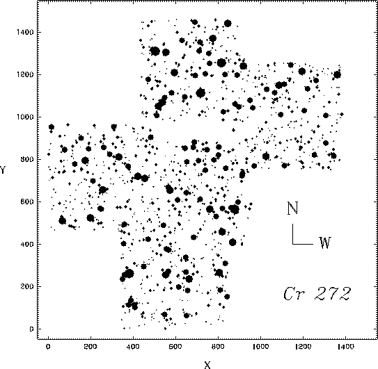
Figure 2: The finding chart of Cr 272. The size of the dots
is proportional to the star magnitudes, approximately

Figure 3: a-e). The color and magnitude errors from DAOPHOT as a
function of the V magnitude
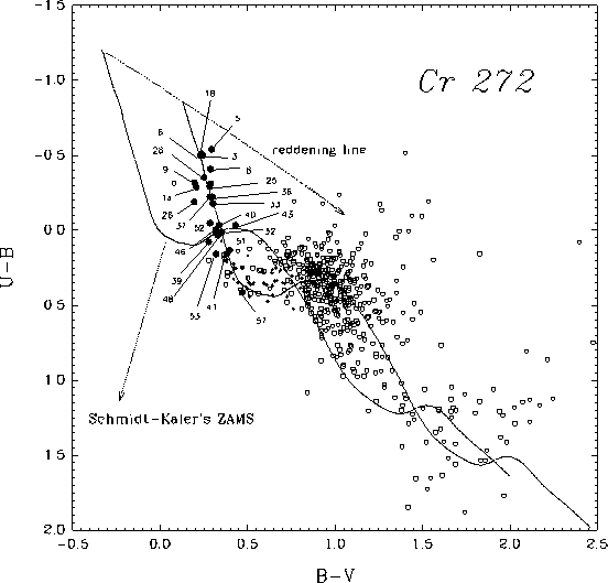
Figure 4: The two-color diagram of Cr 272. Big dots denote likely cluster
members. Small dots are probable members found by comparison among the
photometric diagrams. Squares are stars for which no realistic
memberships could be determined. The solid line is the
Schmidt-Kaler (1982) ZAMS of stars of luminosity class V and the path of the
reddening line ![]() is indicated with
an arrow. Numbers give the star identification
is indicated with
an arrow. Numbers give the star identification
Although the night 8/9 seemed to be veiled, the mean seeing of the
observing runs was ![]()
![]() . To investigate how the field
stars
contaminate the cluster area, a comparison frame was
taken at 30 arcmin from the center of Cr 272 on May 1995 using the same
equipment.
. To investigate how the field
stars
contaminate the cluster area, a comparison frame was
taken at 30 arcmin from the center of Cr 272 on May 1995 using the same
equipment.
PSF fitting using DAOPHOT (Stetson 1987) running within IRAF was employed to get photometry. Previously, the frames were bias subtracted and flat-fielded. Final colors and magnitudes were obtained using two well defined sequences in the clusters NGC 5606 and Hogg 16 (Vázquez & Feinstein 1991a,b) as secondary calibration standards. Most of the calculations were carried out at the Observatory of La Plata but a part of them was preliminary made at the Astronomical Institutes of Bonn University. The rms of the transformation equations have been of the order of 0.01 to 0.02, except in the night 8/9 where the rms reaches up to 0.06. Details of exposure times per filter and night can be found in Table 1 (click here).
|
Filter | Exposure | 1992 (April) | 1994 (April) | ||||
|
| 5/6/7 | 8/9 | 9/10 | 11/12 | 12/13 | ||
|
U | long | | | | |
| |
| medium | | ||||||
| short | | | | ||||
|
B | long | | | | |
| |
| medium | | ||||||
| short | | | | | |||
|
V | long | | | | |
| |
| medium | | ||||||
| short | | | | |
| ||
|
R | long | | | | | ||
| medium | | | |||||
| short | | | | | |||
|
I | long | | | | | ||
| medium | | |
| ||||
| short | | | | | |||
|
| |||||||
Note:
The columns give the ![]()

Figure 5: a) The V vs. B-V color-magnitude diagram. The
Schmidt-Kaler
(1982) Zams is superposed according to the distance modulus obtained in
Sect. 3.2. Symbols as in Fig. 4. b)
The V vs. U-B color-magnitude diagram. Symbols as in Fig. 4

Figure 6: a) The V vs. V-I color-magnitude diagram. Symbols as in
Fig. 4. b)
The B-V vs. V-I diagram. Solid
lines indicate the intrinsic colors for stars of luminosities V and III
according to Cousins (1978). The
dotted lines show the path of the reddening with slopes 1.24 (R=3.1)
(Dean et al. 1978) and 1.45 (R=3.6) respectively
Symbols as in Fig. 4
Table 2 lists 1201 stars with available CCD data containing the identification numbers in Col. 1, x and y coordinates in the second and third columns respectively and magnitudes and colors in the remaining columns. The accuracy of CCD data is given in Figs. 3 (click here)a-e where color and magnitude photometric errors from DAOPHOT are plotted against V.