Among the various iterative methods that can be implemented
for finding an approximation to
the image (or the object) to be reconstructed,
there exists a very slow algorithm
which is based on a matching pursuit strategy.
As will be clarified in this section,
this algorithm is nothing but
an aborted version of a particular algorithm
minimizing q on ![]() (see the introduction of Sect. 1.1).
The corresponding iterative process must never be used in practice
for solving the problem.
Its slow convergence may however be of interest
for initializing the choice of
the object representation space E .
It is therefore important to analyse its principle
(Sect. 2.1),
and in particular, to show that CLEAN is an algorithm of this type
(Sect. 2.2).
(see the introduction of Sect. 1.1).
The corresponding iterative process must never be used in practice
for solving the problem.
Its slow convergence may however be of interest
for initializing the choice of
the object representation space E .
It is therefore important to analyse its principle
(Sect. 2.1),
and in particular, to show that CLEAN is an algorithm of this type
(Sect. 2.2).
Let ![]() be the virtual data vector
corresponding to the object atom
be the virtual data vector
corresponding to the object atom ![]() (cf. Sect. 1.1),
and
(cf. Sect. 1.1),
and
![]() be the projection (operator) of
be the projection (operator) of ![]() onto
the space generated by
onto
the space generated by ![]() :
:
![]()
where
![]()
The guiding idea
is to determine the projection of ![]() onto
onto ![]() via
the elementary projections
via
the elementary projections ![]() .
.
Let us consider the iteration
in ![]() :
:
![]()
![]() is a relaxation parameter to be defined.
At each iteration,
is a relaxation parameter to be defined.
At each iteration,
![]() is chosen so that
is chosen so that
![]()
If
![]() ,
then
,
then
![]() (the projection of
(the projection of ![]() onto
onto ![]() )
and the problem is solved.
)
and the problem is solved.
Let us set
![]() and
and
![]() .
As
.
As
![]() ,
we have from Eq. (21):
,
we have from Eq. (21):
![]()
It follows that
![]()
hence
![]()
Likewise,
![]() .
Provided that
.
Provided that ![]() lies in the open interval (0, 2) ,
lies in the open interval (0, 2) ,
![]() is strictly positive.
Then,
is strictly positive.
Then,
![]() .
The sequence
.
The sequence ![]() ,
where
,
where ![]() ,
therefore converges towards some nonnegative
number
,
therefore converges towards some nonnegative
number ![]() .
As shown in Appendix 2,
.
As shown in Appendix 2,
![]() proves to be equal to 0.
As a result,
proves to be equal to 0.
As a result,
![]()
![]() .
The iterates (21) then converge
towards
.
The iterates (21) then converge
towards ![]() .
.
The maximal value of ![]() is attained for
is attained for
![]() .
To increase the convergence speed of the projection
.
To increase the convergence speed of the projection ![]() ,
,
![]() may be set equal to this optimal value.
The corresponding algorithm,
may be set equal to this optimal value.
The corresponding algorithm,
![]() ,
is nothing but a traditional matching pursuit process
(see Mallat & Zhang 1993).
,
is nothing but a traditional matching pursuit process
(see Mallat & Zhang 1993).
As ![]() ,
we have from Eq. (19),
,
we have from Eq. (19),
![]()
hence
![]()
where
![]() .
The relaxed matching pursuit iteration (21)
can therefore be written in the form
.
The relaxed matching pursuit iteration (21)
can therefore be written in the form
![]()
Clearly, this sequence is the image by A
of the object sequence (in ![]() ):
):
![]()
where
![]()
According to its definition,
the residue ![]() is obtained via the iteration:
is obtained via the iteration:
![]()
As, from Eqs. (24) and (26),
![]() ,
we have (cf. Eq. (20)):
,
we have (cf. Eq. (20)):
![]()
On setting (cf. Eq. (1))
![]()
it follows from Eq. (23) that ![]() is obtained
through the iteration:
is obtained
through the iteration:
![]()
Provided that ![]() lies in the open interval (0, 2) ,
the iterates
lies in the open interval (0, 2) ,
the iterates ![]() converge towards
the minimal value of q on
converge towards
the minimal value of q on ![]() .
Sequence (25) then converges towards a solution
.
Sequence (25) then converges towards a solution ![]() of the problem;
of the problem; ![]() is the
unique solution
is the
unique solution ![]() ,
if and only if
,
if and only if ![]() is a one-to-one map.
is a one-to-one map.
In our formulation of ÇLEAN|,
which essentially follows that of Högbom (1974),
the object space is the ![]() space
space ![]() introduced in Sect. 1.2.
The vectors
introduced in Sect. 1.2.
The vectors ![]() are then
translated versions of the clean beam
are then
translated versions of the clean beam
![]() (see Fig. 3 (click here)b).
More precisely, the elements of
(see Fig. 3 (click here)b).
More precisely, the elements of ![]() are the clean beams
are the clean beams ![]() centred on the nodes of
the
"clean box"
centred on the nodes of
the
"clean box" ![]() :
:
![]()
The data space ![]() coincides with the experimental data space
coincides with the experimental data space ![]() ,
and A with
the experimental Fourier sampling operator:
,
and A with
the experimental Fourier sampling operator:
![]() on
on ![]() .
As the image to be reconstructed is defined as the
convolution of the original object by the clean beam (Eq. (13)),
the data vector
.
As the image to be reconstructed is defined as the
convolution of the original object by the clean beam (Eq. (13)),
the data vector ![]() must be defined as the experimental data vector
must be defined as the experimental data vector ![]() damped by the Fourier transform of the clean beam:
damped by the Fourier transform of the clean beam:
![]() (cf. Eq. (14)).
We then have
(cf. Eq. (14)).
We then have ![]() with (cf. Eqs. (1), (12) and (17)):
with (cf. Eqs. (1), (12) and (17)):
![]()
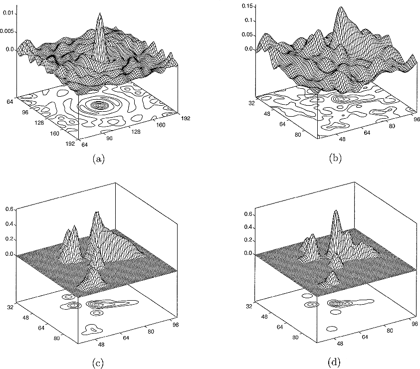
Figure 5: Image reconstruction via CLEAN with ![]() ;
a) dirty beam;
b) dusty map;
c) image to be reconstructed (Fig. 4 (click here));
d) clean map for
;
a) dirty beam;
b) dusty map;
c) image to be reconstructed (Fig. 4 (click here));
d) clean map for ![]() (the definition of the fit criterion
(the definition of the fit criterion ![]() is given in Eq. (35)).
In the conditions of this simulation
(see Fig. 3 (click here)),
the optimal fit threshold of CLEAN is of the order of 1.75.
For a lower threshold,
the support of the clean map
is no longer contained in that of the image to be reconstructed.
In the framework of the analysis presented in this paper,
the residual maps
is given in Eq. (35)).
In the conditions of this simulation
(see Fig. 3 (click here)),
the optimal fit threshold of CLEAN is of the order of 1.75.
For a lower threshold,
the support of the clean map
is no longer contained in that of the image to be reconstructed.
In the framework of the analysis presented in this paper,
the residual maps ![]() or
or ![]() must not be added to the clean map
must not be added to the clean map
As explicitly shown in Appendix 3,
the "dirty map" is the map of the scalar components
of ![]() in the basis of the elementary particles
in the basis of the elementary particles ![]() .
In this context,
.
In this context,
![]() may be referred to as the "dusty map".
For clarity, we set
may be referred to as the "dusty map".
For clarity, we set
![]() and
and
![]() .
Likewise,
the action of
.
Likewise,
the action of ![]() corresponds to a
"discrete convolution" by the "dirty beam"
corresponds to a
"discrete convolution" by the "dirty beam" ![]() :
:
![]() (the precise definition of this operation is given in Appendix 3).
Thus, from Eq. (20),
the parameters
(the precise definition of this operation is given in Appendix 3).
Thus, from Eq. (20),
the parameters ![]() are all equal to:
are all equal to:
![]()
The relaxed matching pursuit iteration (25) can then be written in the form
![]()
where (from Eq. (26))
![]()
Clearly, ![]() (the map of the
(the map of the ![]() )
is nothing but the "discrete intercorrelation" of
)
is nothing but the "discrete intercorrelation" of ![]() with CB.
with CB.
The residue ![]() and the quadratic errors
and the quadratic errors ![]() are respectively obtained via the iterations (27) and (28):
are respectively obtained via the iterations (27) and (28):
![]()
and
![]()
Note that
![]() .
.
In the classical presentation of ÇLEAN|,
the convolution by the clean beam is performed
a posteriori, whence some small differences in
these iterations
(cf. Appendix 4).
In particular,
in the version of ÇLEAN| presented here,
![]() is chosen (at each iteration) so that
is chosen (at each iteration) so that
![]() .
.
The process is interrupted as soon
as ![]() is less than a threshold value
related to the level of the noise in the Fourier domain.
In our implementation of ÇLEAN|,
we introduce the "fit criterion" (cf. Eqs. (18) and (29)):
is less than a threshold value
related to the level of the noise in the Fourier domain.
In our implementation of ÇLEAN|,
we introduce the "fit criterion" (cf. Eqs. (18) and (29)):
![]()
As soon as ![]() is less than 2 (for example),
the matching pursuit process is interrupted;
is less than 2 (for example),
the matching pursuit process is interrupted;
![]() is the corresponding "clean map".
is the corresponding "clean map".
In the simulation presented in Fig. 5 (click here),
we show the clean map corresponding to the fit threshold 2 .
The relaxation parameter ![]() was set equal to 0.2 ,
and the clean box was defined as the support of
was set equal to 0.2 ,
and the clean box was defined as the support of ![]() at a lower level of resolution (twice as low).
In the conditions of this simulation,
the optimal fit threshold of CLEAN is of the order of 1.75.
For a lower threshold, the support of the clean map
is no longer contained in that of the image to be reconstructed.
at a lower level of resolution (twice as low).
In the conditions of this simulation,
the optimal fit threshold of CLEAN is of the order of 1.75.
For a lower threshold, the support of the clean map
is no longer contained in that of the image to be reconstructed.
Let E be the object representation space
generated by the ![]() selected by ÇLEAN|.
Clearly,
the clean map
selected by ÇLEAN|.
Clearly,
the clean map ![]() does not minimize
does not minimize ![]() on E .
The same matching pursuit
algorithm (with
on E .
The same matching pursuit
algorithm (with ![]() )
can be confined to E for performing
the complete minimization on this space.
This corresponds to the principle of what is referred to as "Window ÇLEAN|"
(Schwarz 1978).
The algorithms presented in Sects. 3 and 4
are much more efficient for this purpose,
but as specified in Sect. 5,
they only reveal that
(in situations of astrophysical interest)
the solution thus obtained is without any interest:
the problem is ill-conditioned.
)
can be confined to E for performing
the complete minimization on this space.
This corresponds to the principle of what is referred to as "Window ÇLEAN|"
(Schwarz 1978).
The algorithms presented in Sects. 3 and 4
are much more efficient for this purpose,
but as specified in Sect. 5,
they only reveal that
(in situations of astrophysical interest)
the solution thus obtained is without any interest:
the problem is ill-conditioned.