We have followed Schmid in using Monte-Carlo techniques to model the line formation. This is in part because the Raman line-formation process is a multi-scattering problem, and does not lend itself easily to an analytical treatment; but also because the flexibility which the Monte-Carlo approach offers in formulating different versions of the model. The problem is therefore simply one of generating source OVI photon packets and following the subsequent interaction of this radiation with the red-giant wind.
The model consists of a giant star, radius ![]() , which is centred
at the origin of the Cartesian frame, and a source of the parent photons
which is centred on the x-axis at a distance
, which is centred
at the origin of the Cartesian frame, and a source of the parent photons
which is centred on the x-axis at a distance ![]() from the
origin. The observer is located in the xy-plane, with the z-axis
perpendicular to the line-of-sight. (This entails no loss of
generality; the xy plane need not be the orbital plane.)
from the
origin. The observer is located in the xy-plane, with the z-axis
perpendicular to the line-of-sight. (This entails no loss of
generality; the xy plane need not be the orbital plane.)
The giant star has an extended atmosphere which is assumed to be
spherically symmetric. For a mass-losing star the density structure is
defined by the stellar mass-loss rate ![]() and a velocity structure
v(r) through the equation of mass conservation:
and a velocity structure
v(r) through the equation of mass conservation:
![]()
Other structures (e.g., extended, hydrostatic atmospheres) are trivially
substituted.
A photon packet is fully described by its frequency ![]() , position
, position
![]() , direction
, direction ![]() , and normalized linear Stokes
vector
, and normalized linear Stokes
vector
![]() , where w is the weight (initially
, where w is the weight (initially
![]() ). The total Stokes parameters for N photon packets are
). The total Stokes parameters for N photon packets are
![]()
The Stokes parameters are calculated with respect to the meridional plane containing the photon path and the z-axis, so the upper-lower symmetry of the system about the line-of-centres means that the U Stokes parameter cancels in the integrated spectrum.
For most models we assumed a point source of OVI
photons (trial calculations for an extended source are reported in
Sect. 11 (click here)). We assume that the emission is isotropic, so that
the initial direction of the photon packet may be obtained from
![]()
![]()
![]()
where
![]()
![]()
and ![]() is a uniform random deviate in the range 0-1.
is a uniform random deviate in the range 0-1.
In principle, a weighting scheme could be used to bias the initial direction of the photon packet towards the red-giant component (while retaining the assumption of intrinsically isotropic emission). We experimented with such schemes, which can improve the statistical efficiency of the calculation, but found that the high weights given to the relatively few packets emitted in the direction away from the red giant, modified by the weighting schemes discussed below, gave cosmetically unsatisfactory results for relatively small savings in computer time.
The radiation from the source region is assumed to be
initially unpolarized, so
that the position angle ![]() of a source photon packet is given by
of a source photon packet is given by
![]()
The probability of a collision event (scattering or absorption) is
defined by the optical depth ![]() , where the probability density
function for an event is
, where the probability density
function for an event is
![]()
The normalized cumulative probability function is
![]()
where ![]() is the optical depth to the collision. Using the inverse
transform method gives
is the optical depth to the collision. Using the inverse
transform method gives
![]()
Once the optical depth from the photon source to the
event has been obtained, the physical path length to the event is
calculated. The optical depth is the integral
![]()
where l is the path length, ![]() the density, and
the density, and ![]() the total opacity. By inverting this integral
equation it is possible to obtain the path length for a given
optical depth; the inversion can be carried out analytically for
a number of simple density distributions.
the total opacity. By inverting this integral
equation it is possible to obtain the path length for a given
optical depth; the inversion can be carried out analytically for
a number of simple density distributions.
The absorption cross-section for the OVI photons,
![]() , and the absorption cross-section for the
Raman-scattered
photons,
, and the absorption cross-section for the
Raman-scattered
photons, ![]() , may be calculated in principle, but
here are
treated as free parameters, specified in units of the total
scattering cross-section
, may be calculated in principle, but
here are
treated as free parameters, specified in units of the total
scattering cross-section ![]() , where
, where
![]()
and where ![]() and
and ![]() are the Rayleigh-
and
Raman-scattering cross-sections, respectively. All these quantities
(especially the absorption cross-sections)
are wavelength-dependent, but we adopt representative
monochromatic
values at the line wavelengths; in particular, we use Raman and Rayleigh
scattering cross-sections from Schmid (1989).
are the Rayleigh-
and
Raman-scattering cross-sections, respectively. All these quantities
(especially the absorption cross-sections)
are wavelength-dependent, but we adopt representative
monochromatic
values at the line wavelengths; in particular, we use Raman and Rayleigh
scattering cross-sections from Schmid (1989).
Since better statistics are obtained as more Raman photons escape to the
observer, it is inefficient to lose photons through absorption. We
therefore employ a variance-reduction technique in which all photon
packets are forced to scatter. To conserve intensity, the photon
packets are re-weighted at each scattering by a factor
![]()
where ![]() is the scattering optical depth,
is the scattering optical depth, ![]() is the
absorption optical depth and
is the
absorption optical depth and ![]() is the total (absorption plus
scattering) collision cross-section.
is the total (absorption plus
scattering) collision cross-section.
For additional efficiency, all OVI photons are forced to
scatter before reaching the system boundary (which is taken as
1000![]() in the numerical models presented here);
i.e.,
all OVI photons are converted to Raman photons. If
in the numerical models presented here);
i.e.,
all OVI photons are converted to Raman photons. If
![]() is the optical depth to the system boundary then the
optical depth to scattering,
is the optical depth to the system boundary then the
optical depth to scattering, ![]() , is
, is
![]()
and the photon weight, w, is adjusted by a factor
![]()
A comprehensive account of radiation transfer according to the Rayleigh-scattering phase matrix is given by Chandrasekhar (1960). The geometry for the scattering event is given in Fig. 1 (click here).
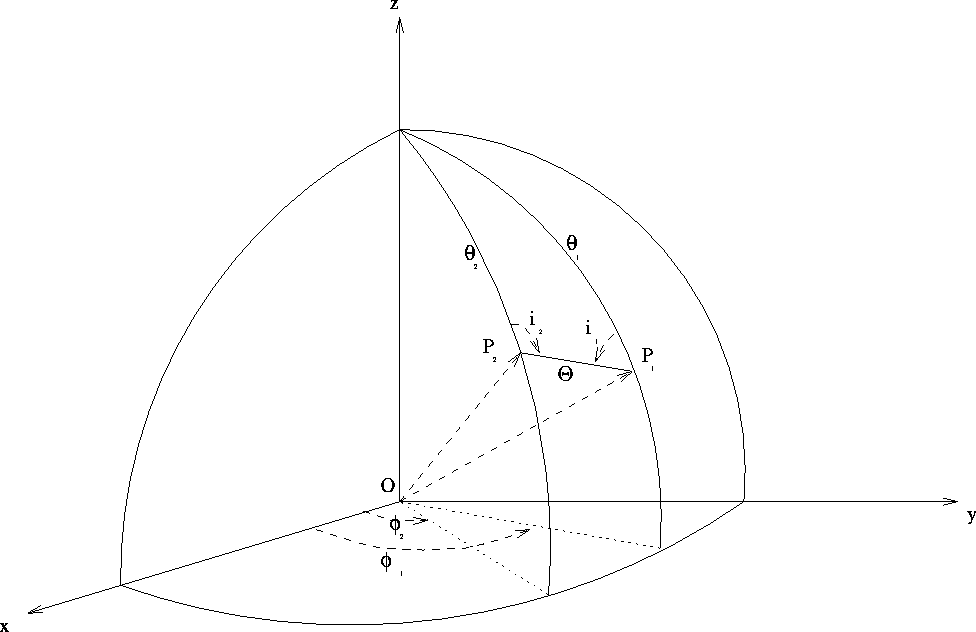
Figure 1: The geometry of a scattering event. The photon packet
encounters the scatterer at O, entering while
travelling in the direction ![]() and exiting in the direction
and exiting in the direction
![]() , having been
scattered through an angle
, having been
scattered through an angle ![]()
The photon packet, initially travelling in direction ![]() , is
scattered
through an angle
, is
scattered
through an angle ![]() and exits the scattering event travelling in
direction
and exits the scattering event travelling in
direction ![]() . The Stokes parameters of the incoming photon beam refer
to the meridian plane
. The Stokes parameters of the incoming photon beam refer
to the meridian plane ![]() . In order to calculate the resultant
polarization the Stokes parameters must be rotated though an angle
. In order to calculate the resultant
polarization the Stokes parameters must be rotated though an angle
![]() in order that they refer to the scattering plane
in order that they refer to the scattering plane ![]() . The
rotation matrix
. The
rotation matrix ![]() that rotates the Stokes parameters through a
clockwise angle
that rotates the Stokes parameters through a
clockwise angle ![]() is
is
Thus the Stokes vector relative to the scattering plane, ![]() ,
is given by
,
is given by
![]()
where

Both Raman and Rayleigh scatterings occur according to the
Rayleigh-scattering phase matrix ![]() , where
, where
and ![]() is the scattering angle. Once the phase matrix has been applied,
the Stokes vector must be rotated by
is the scattering angle. Once the phase matrix has been applied,
the Stokes vector must be rotated by ![]() so that it refers to the
meridian plane
so that it refers to the
meridian plane ![]() . Thus the Stokes vectors of the incident and scattered
beam,
. Thus the Stokes vectors of the incident and scattered
beam, ![]() and
and ![]() , are related by
, are related by
![]()
where ![]() is the scattering cross-section.
is the scattering cross-section.
If ![]() is the azimuthal scattering angle measured relative to the
plane of scattering then the cumulative probability distribution of
the scattering angles
is the azimuthal scattering angle measured relative to the
plane of scattering then the cumulative probability distribution of
the scattering angles ![]() is obtained by integrating
the Stokes I component over all solid angles. Hence
is obtained by integrating
the Stokes I component over all solid angles. Hence
![]()
This two-dimensional equation must be decomposed into two
one-dimensional equations (cf. Schmid 1992). Integrating
Eq. (21 (click here)) over ![]() gives the cumulative probability
distribution function
gives the cumulative probability
distribution function
![]()
while
integrating over ![]() , and using the
normalization
, and using the
normalization
![]()
gives the cumulative probability distribution function
![]()
The inverse-transform method was used to set up look-up tables of
![]() . For Rayleigh-scattering events, the new photon
direction with respect to the scattering plane is found from
interpolation in these tables. The new photon-packet direction in the
Cartesian frame is then obtained from trigonometric relations. The
polarization with respect to the new photon-packet direction is obtained
by applying Eq. (20 (click here)) to the incident polarization vector.
The intensity component of the Stokes vector is not altered, as the
intensity distribution of the phase matrix is included in the choice of
photon-packet direction.
. For Rayleigh-scattering events, the new photon
direction with respect to the scattering plane is found from
interpolation in these tables. The new photon-packet direction in the
Cartesian frame is then obtained from trigonometric relations. The
polarization with respect to the new photon-packet direction is obtained
by applying Eq. (20 (click here)) to the incident polarization vector.
The intensity component of the Stokes vector is not altered, as the
intensity distribution of the phase matrix is included in the choice of
photon-packet direction.
When a Raman-scattering event occurs, the photon packet is forced to
scatter towards the observer. The new polarization vector is again
found by applying Eq. (20 (click here)). The photon packet must be
weighted by the probability that it is scattered towards to observer, so
that the final weight of a packet at the nth scattering is
![]()
where ![]() and
and ![]() are given by Eqs. (13 (click here))
and (15 (click here)),
are given by Eqs. (13 (click here))
and (15 (click here)), ![]() is the scattering angle, and
is the scattering angle, and ![]() refers to the scattering plane.
refers to the scattering plane.
For most of the models discussed here, the OVI emitters are assumed to have zero mean velocity in the binary reference frame. (We neglect the dynamical effects of orbital motion, since orbital velocities are likely to be smaller than wind velocities for all but the shortest-period, slowest-wind systems.)
Scattering events in the expanding wind subsequently introduce frequency
shifts through the Doppler effect.
If ![]() is the
direction of the incident photon packet,
is the
direction of the incident photon packet, ![]() is the
direction
of the scattered beam, and
is the
direction
of the scattered beam, and ![]() is the velocity of the
scattering particle, then the frequency of the incident photon
packet with respect to the rest frame of the scatterer is
is the velocity of the
scattering particle, then the frequency of the incident photon
packet with respect to the rest frame of the scatterer is
![]()
where ![]() is the frequency of the photon packet in
the observer's rest frame.
Once the frequency is put in the rest frame of the scatterer, any
frequency shift introduced by the Raman scattering may be calculated. The
frequency of the Raman-scattered photon packet is given by
is the frequency of the photon packet in
the observer's rest frame.
Once the frequency is put in the rest frame of the scatterer, any
frequency shift introduced by the Raman scattering may be calculated. The
frequency of the Raman-scattered photon packet is given by
![]()
where ![]() is the rest frequency of Ly
is the rest frequency of Ly![]() . The
frequency can then be converted back to the observer's rest frame:
. The
frequency can then be converted back to the observer's rest frame:
![]()
In a constant-velocity-wind model (for example) there
is a finite density at the wind base, and under these circumstances
photon packets may reach the red-giant surface without scattering.
To treat this case we use
a `core-halo' model of an extended wind and a thin, static
photosphere; we
treat transfer in the photosphere
in a locally plane-parallel geometry.
The photon packet is incident on the photosphere
at an angle ![]() to the normal,
to the normal, ![]() . The optical
depth to scattering,
. The optical
depth to scattering, ![]() , is determined and the vertical optical
depth,
, is determined and the vertical optical
depth, ![]() , is stored, where
, is stored, where
![]()
The photon packet is then scattered.
If it is Raman scattered, then it goes to the
observer in the normal way. If it is Rayleigh
scattered, then the
new direction and polarization of the packet is found from the phase
matrix, and the
optical depth to the next scattering determined. The angle of the
photon-packet direction with respect to the normal is calculated from
![]()
where ![]() is the direction of the packet. The vertical
optical depth is then recalculated according to
is the direction of the packet. The vertical
optical depth is then recalculated according to
![]()
If the new vertical optical depth is negative then the photon has
escaped, and the next scattering is performed in the wind.