2 Observations and data reduction

As a basis for our database we have taken the flux density measurements published by Lorimer et al. (1995). These observations were made between July 1988 and October 1992 using the 76-m Lovell radio telescope at Jodrell Bank, at frequencies 408, 606, 925, 1408 and 1606 MHz. Lorimer et al. (1995) excluded from their sample those pulsars which were too weak to obtain reliable flux density measurements as well as the millisecond pulsars. We have extended this database by observations made at higher frequencies by different authors mentioned earlier or those unpublished but made available at MPIfR archives in Bonn. All observations at frequency range from 1.4 GHz to 43 GHz were made with the 100-m radio telescope of the MPIfR at Effelsberg and are available in European Pulsar Network Database (Lorimer et al. 1998). Some values at 1.4 and 1.6 GHz were also published by Lorimer et al. (1995). We performed additional observations at 4.85 GHz of 43 very weak pulsars in August 1998. We managed to detect 30 objects and those undetected are listed in Table 1. The detection limit of $S\sim 0.05$ mJy for the survey published by Kijak et al. (1998) is clearly visible from this table. The observations published by Izvekova et al. (1981) and Malofeev et al. (2000) were performed at the Pushchino Radio Astronomical Observatory of the Lebedev Physical Institute.

 

 

Table 1: Pulsars not detected at 4.85 GHz. The pulsar name, total observing time and upper limits $S_{\rm max}$ for the total flux density are listed

PSR B	Time	$S_{\rm max}$	PSR B	Time	$S_{\rm max}$
	[min]	[mJy]		[min]	[mJy]
0621-04	30	0.02	1820-14	20	0.02
1246+22	50	0.01	1834-04	30	0.01
1534+12	20	0.01	1839-04	25	0.03
1600-27	25	0.01	1848+12	20	0.01
1811+40	20	0.01	2210+29	100	0.01
1813-17	25	0.01	2323+63	20	0.03

2.1 Calibration procedure

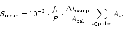
In order to calibrate the flux density of a pulsar using a system in the Effelsberg Radio-observatory, a noise diode installed in every receiver is switched synchronously with the pulse period. The energy output for the noise diode is then compared with energy received from the pulsar, since the first samples of an observed pulse profile contain the calibration signal while the remaining samples contain the pulse. The energy of the noise diode itself can be calibrated by comparing its output to the flux density of a known continuum sources. This pointing procedure is generally performed on well known reliable flux calibrators, e.g. 3C 123, 3C 48, etc. From these pointing observations a factor $f_{{\rm c}}$ translating the height of the calibration signal into flux units, is derived. The energy of a pulse is given as the integral beneath its waveform which in arbitrary units yields

$$E=\sum\limits_{i\in {\rm pulse}}A_{i}\Delta t_{{\rm samp}}=\Delta t_{{\rm samp}} \sum\limits_{i\in {\rm pulse}}A_{i}$$ (1)

where A_i is the pulse amplitude measured in the phase bin i and $\Delta t_{{\rm {samp}}}$ is the sampling time. Scaling the whole profile now in units of the height of the calibration signal measured in the same profile, $A_{{\rm cal}}$, we obtain

$$E=\Delta t_{{\rm samp}}\sum\limits_{i\in {\rm pulse}}\frac{A_{i}}{A_{{\rm {cal}}}}\cdot$$ (2)

Using the conversion factor $f_{{\rm c}}$, the mean pulse energy is translated into proper units, i.e. $\rm J~m^{-2}~Hz$, according to the following formula

$$E=f_{{\rm c}}\cdot\frac{\Delta t_{{\rm samp}}}{A_{{\rm cal}}}\sum\limits_{i\in {\rm pulse}} A_{i} .$$ (3)

The mean flux represents the pulse energy averaged over a pulse period,

$$S_{{\rm mean}}=\frac{E}{P}\cdot$$ (4)

Finally, assuming that $f_{{\rm c}}$ converts the units of the calibration signal strength into mJy, and the sampling time $\Delta t_{{\rm {samp}}}$ is given in $\mu$s, the mean flux is obtained as (Kramer 1995)

$$S_{{\rm mean}}=10^{-3}\cdot\frac{f_{{\rm c}}}{P}\cdot\frac{\D... ...rm samp}}}{A_{{\rm cal}}}\sum\limits_{i\in {\rm pulse}}A_{i} .$$ (5)

2.2 Error analysis

Pulsars are generally known to be stable radio sources although the measured flux density varies due to diffractive and refractive scintillation effects (e.g. Stinebring & Condon 1990). Interstellar scintillations are caused by irregularities in the electron density of the interstellar medium. The observed flux variations are frequency and distance dependent and also depend on the observing set-up, i.e. on the relative width of observing and scintillation bandwidth (e.g. Malofeev et al. 1996; Malofeev 1996). Unless the receiver bandwidth is significantly larger than the scintillation bandwidth, which increases with frequency, strong variations in the observed flux densities are to be expected. Usually, however, the amplitude of scintillation decreases towards higher frequencies, so that those data are less influenced by the scintillation effects. Nevertheless, the question of intrinsic variations on very short and very long time scales remains still open (cf. Stinebring & Condon 1990). Assessing the situation is hampered by the fact that many authors do not estimate the always present influence of interstellar scintillations or do not quote error estimates at all. Given the difference in the observing set-ups for given observatories, a careful analysis is difficult. We try to circumvent this unpleasant situation by estimating errors for the pulsar flux densities in our sample from published values, wherever available, and standard deviations of the average of single measurements. If only one measurement was available, an error estimate could not be computed although it may happen that form of the spectrum changes when new measurements are added.

2.3 Search technique for break frequency

Since a robust theory of pulsar radio emission does not exist, the true shape of pulsar spectra is still not known. A fair first attempt is to model them by simple power laws. Previous studies (e.g. Sieber 1973; Malofeev et al. 1994) showed however that some pulsar spectra cannot apparently be described by this simple approach. Usually, such a conclusion is reached after a visual inspection of the data, i.e. after a power law fit has been done. However, if pulsar spectra are indeed more complicated, the usual next step to fit a composite (or "broken'') power law is just another approximation, where the undersampling of the spectrum in the observed range of frequencies would place any fitted "break'' naturally in the range of a few GHz, i.e. the range where they are indeed usually observed as it was clearly pointed out by Thorsett (1991). Nevertheless, even if two power laws are just another approximation to a "true'' spectrum, any need to fit a break in order to describe the data adequately would represent a valuable hint on the true nature of pulsar spectra. It is therefore very important to search for such breaks in the spectra, while keeping just discussed limitations in mind. We believe, however, that one has to be more quantitative when describing the need for fitting a two power laws rather than a simple power law. This is even more important in the light of the latest results on millisecond pulsar spectra (Kramer et al. 1999; Kuzmin & Losovski 2000), where no significant break (not even a low frequency turn-over) has been found. Hence, we adopted in this work the following approach: firstly, we fitted a simple power law to the flux density data, assuming that this describes the data sufficiently. We calculated a $\chi^2$ and the probability Q that a random $\chi^2$ exceeds this value for a given number of degrees of freedom. These computed probabilities give a quantitative measure for the goodness-of-fit of the model. If Q is very small then the apparent discrepancies are unlikely to be chance fluctuations. Much more probably either the model is wrong, or the measurement errors are larger than stated, or measurement errors might not be normally distributed. Generally, one may accept models with $Q \sim$ 0.001 (Press et al. 1996). Secondly, we assumed that a two power law had to be fitted to the data, using the following rules:

$$S(\nu) = \left \{ \begin{array}{r@{:\quad}l} c_1 \nu^{\alpha... ...c_2 \nu^{\alpha_2} & \nu > \nu_{\rm b}\, . \end{array} \right.$$ (6)

Since the break frequency, $\nu _{\rm b}$, is a priori unknown, we treated it as a free parameter and tried to minimize a corresponding $\chi^2$ simultaneously over the whole parameter space of $c_1,~c_2,~\alpha_1, ~\alpha_2$ and $\nu _{\rm b}$. Due to the nature of the additional boundary condition ( $\nu\le\nu_{\rm b}$ or $\nu>\nu_{\rm b}$), we applied a Simplex algorithm as described by Nelder & Mead (1965). For the resulting, minimized $\chi^2$ we then calculated again the probability that a random $\chi^2$ is larger than the found value. A comparison of the $\chi^2$-statistics for both cases was then used to judge whether a break was truly significant or not. The fitting procedure was performed on data in the frequency range from 400 MHz to 23 GHz. We have not taken into account data corresponding to single measurements, as well as those at frequencies lower than 400 MHz, as they could represent a low frequency turn-over which usually occurs at $\sim$ 100 MHz. There is a gap in data coverage between 100 and 300 MHz, but this should not affect our analysis and conclusions.

 

 

Table 2: Spectral indices for 266 pulsars with simple power-law spectrum $S\sim \nu ^{\alpha }$ calculated for a given frequency range with error and a probability of the goodness-of-fit Q (see text)

PSR B	Freq. range	$\alpha$	$\sigma_\alpha$	Q		PSR B	Freq. range	$\alpha$	$\sigma_\alpha$	Q
	[GHz]
0011+47	0.4 - 4.9	-1.3	0.10	8.3E-01		0950+08	0.4 - 10.6	-2.2	0.03	1.7E-02
0031-07	0.4 - 10.7	-1.4	0.11	4.1E-03		1010-23	0.4 - 0.6	-1.9
0037+56	0.4 - 4.8	-1.8	0.05	6.3E-03		1016-16	0.4 - 1.4	-1.7	0.28	9.1E-01
0045+33	0.4 - 1.4	-2.5	0.26			1039-19	0.4 - 1.4	-1.5	0.28	6.8E-01
0052+51	0.4 - 1.4	-0.7	0.14	6.1E-01		1112+50	0.4 - 4.9	-1.7	0.11	6.0E-02
0053+47	0.4 - 4.9	-1.6	0.09			1133+16	0.4 - 32.0	-1.9	0.06	7.4E-02
0059+65	0.4 - 1.6	-1.6	0.13	1.4E-01		1254-10	0.4 - 1.6	-1.8	0.16	6.4E-01
0105+65	1.4 - 1.4	-1.9	0.19	4.3E-01		1309-12	0.4 - 1.4	-1.7	0.16	2.8E-01
0105+68	0.4 - 1.4	-1.8	0.22			1322+83	0.4 - 1.4	-1.6	0.30	8.7E-01
0114+58	0.4 - 1.4	-2.5	0.21	8.5E-01		1508+55	0.4 - 4.9	-2.2	0.07	5.2E-02
0138+59	0.4 - 1.4	-1.9	0.16	7.0E-01		1530+27	0.4 - 4.9	-1.4	0.10	1.3E-01
0144+59	0.4 - 14.6	-1.0	0.04	6.1E-04		1540-06	0.4 - 4.9	-2.0	0.11	4.0E-02
0148-06	0.4 - 1.4	-2.7	0.58	4.6E-01		1541+09	0.4 - 4.9	-2.6	0.04	2.7E-03
0149-16	0.4 - 1.4	-2.1	0.26	2.3E-01		1552-23	0.4 - 4.9	-1.8	0.08	1.1E-02
0153+39	0.4 - 0.6	-2.2				1552-31	0.4 - 1.4	-1.6	0.19	3.0E-04
0154+61	0.4 - 1.4	-0.9	0.12	1.4E-03		1600-27	0.4 - 1.4	-1.7	0.13	4.0E-04
0320+39	0.4 - 1.4	-2.9	0.24	5.2E-01		1604-00	0.4 - 4.9	-1.5	0.08	6.8E-01
0329+54	1.4 - 23.0	-2.2	0.03	7.5E-04		1607-13	0.4 - 0.6	-2.1	0.45
0331+45	0.4 - 1.4	-1.9	0.24	1.5E-01		1612+07	0.4 - 1.4	-2.6	0.30	1.7E-01
0339+53	0.4 - 1.4	-2.2	0.28	2.5E-02		1612-29	0.4 - 0.6	-0.8	0.98
0353+52	0.4 - 1.4	-1.6	0.12	7.4E-01		1620-09	0.4 - 4.9	-1.7	0.13	1.5E-01
0402+61	0.4 - 1.4	-1.4	0.08	1.4E-01		1633+24	0.4 - 1.4	-2.4	0.31
0410+69	0.4 - 1.4	-2.4	0.13	8.1E-04		1642-03	0.4 - 10.6	-2.3	0.05	6.7E-01
0447-12	0.4 - 1.4	-2.0	0.11	1.4E-02		1648-17	0.4 - 1.4	-2.5	0.26	5.9E-02
0450+55	0.4 - 4.9	-1.5	0.04	6.0E-02		1649-23	0.4 - 1.4	-1.7	0.09	5.6E-01
0450-18	0.4 - 4.9	-2.0	0.05	2.9E-08		1657-13	0.4 - 0.6	-1.7	0.36
0458+46	0.4 - 1.4	-1.3	0.05	1.2E-05		1700-18	0.4 - 1.4	-1.9	0.23	4.8E-05
0523+11	0.4 - 1.4	-2.0	0.06	1.4E-01		1700-32	0.4 - 0.6	-3.1	0.27
0525+21	0.4 - 4.9	-1.5	0.12	4.4E-01		1702-19	0.4 - 4.9	-1.3	0.05	5.3E-01
0531+21	0.4 - 1.4	-3.1	0.18	5.7E-01		1706-16	0.4 - 32.0	-1.5	0.04	1.1E-01
J0538+2817	1.4 - 4.9	-1.2	0.57			1709-15	0.4 - 4.9	-1.7	0.06	8.7E-01
0559-05	0.4 - 4.9	-1.7	0.04	7.6E-01		1714-34	0.4 - 1.4	-2.6	0.34
0609+37	0.4 - 1.4	-1.5	0.25	3.5E-01		1717-16	0.4 - 4.9	-2.2	0.05	5.7E-01
0611+22	0.4 - 2.7	-2.1	0.04	8.5E-01		1717-29	0.4 - 1.4	-2.2	0.20	8.8E-01
0621-04	0.4 - 1.4	-0.4	0.29	5.0E-01		1718-02	0.4 - 1.4	-2.2	0.16	1.6E-06
0626+24	0.4 - 4.9	-1.6	0.08	1.2E-03		1718-32	0.4 - 1.4	-2.3	0.06	3.9E-01
0628-28	0.4 - 10.6	-1.9	0.10	6.8E-01		1726-00	0.4 - 0.6	-2.3	0.47
0643+80	0.4 - 4.9	-1.9	0.08	2.3E-01		1727-33	0.4 - 1.4	-1.3
0655+64	0.4 - 1.4	-2.1	0.30	1.0E-01		1730-22	0.4 - 1.4	-2.0	0.15	1.4E-01
0656+14	0.4 - 1.4	-0.5	0.17	1.3E-01		1732-07	0.4 - 1.4	-1.9	0.12	1.4E-09
0727-18	0.4 - 1.4	-1.6	0.11	1.3E-02		1734-35	0.6 - 1.4	-1.6	0.30
0740-28	0.4 - 10.6	-2.0	0.03	1.1E-07		1735-32	0.4 - 1.6	-0.9	0.12	2.1E-02
0751+32	0.4 - 4.9	-1.5	0.07	1.8E-01		1736-31	0.6 - 1.6	-0.9	0.20	4.2E-01
0756-15	0.4 - 4.9	-1.6	0.13	6.0E-04		1737+13	0.4 - 4.9	-1.5	0.10	2.8E-01
0809+74	0.4 - 10.6	-1.4	0.06	6.7E-02		1737-30	0.4 - 1.4	-1.3	0.10	4.5E-01
0818-13	0.4 - 4.9	-2.3	0.05	3.4E-01		1738-08	0.4 - 4.9	-2.2	0.08	6.9E-02
0820+02	0.4 - 4.9	-2.4	0.08	9.5E-01		1740-03	0.4 - 1.4	-1.5
0834+06	0.4 - 4.9	-2.7	0.11	2.1E-02		1740-13	0.4 - 1.4	-2.0	0.19	2.3E-02
0853-33	0.4 - 1.4	-2.4	0.20	5.4E-01		1740-31	0.6 - 1.4	-1.9	0.11
0906-17	0.4 - 1.4	-1.4	0.16	2.0E-01		1742-30	0.4 - 4.9	-1.6	0.04	1.5E-06
0917+63	0.4 - 1.4	-1.7	0.37			1745-12	0.4 - 1.4	-2.1	0.12	3.4E-03
0919+06	0.4 - 10.6	-1.8	0.05	7.6E-01		1746-30	0.4 - 1.4	-1.5	0.39
0940+16	0.4 - 1.4	-1.3	0.30	5.3E-01		1747-31	0.6 - 1.4	-1.2	0.31
0942-13	0.4 - 1.4	-3.0	0.30	8.8E-01		1750-24	0.9 - 4.9	-1.0	0.07	1.1E-06
0943+10	0.4 - 0.6	-3.7	0.36			1753+52	0.4 - 4.9	-1.6	0.08	5.8E-04

 

Table 2: continued

PSR B	Freq. range	$\alpha$	$\sigma_\alpha$	Q		PSR B	Freq. range	$\alpha$	$\sigma_\alpha$	Q
	[GHz]
1753-24	0.4 - 1.6	-0.7	0.14	3.2E-01		1845-19	0.4 - 0.6	-2.0	0.46
1754-24	0.4 - 1.4	-1.1	0.09	9.1E-02		1846-06	0.4 - 1.4	-2.2	0.10	8.4E-01
1756-22	0.4 - 4.9	-1.7	0.09	5.3E-01		1848+04	0.6 - 1.4	-1.4
1757-24	0.4 - 0.6	-3.6				1848+12	0.4 - 1.6	-1.9	0.16	4.3E-02
1758-03	0.4 - 1.4	-2.6	0.11	2.3E-01		1848+13	0.4 - 1.6	-1.4	0.18	1.2E-01
1758-23	1.4 - 4.9	-2.5	0.10	8.3E-04		1849+00	1.4 - 4.9	-2.4	0.12	4.8E-01
1800-27	0.4 - 1.4	-1.4				1851-14	0.4 - 0.6	-0.8	0.42
1802-07	0.4 - 1.4	-1.3	0.31			1853+01	0.4 - 0.6	-2.5
1804-08	0.4 - 4.9	-1.2	0.08	6.1E-07		1855+02	0.6 - 4.9	-1.2	0.09	9.5E-02
1804-27	0.6 - 1.4	-3.0	0.21			1857-26	0.4 - 10.7	-2.1	0.06	1.2E-03
1805-20	0.6 - 4.9	-1.5	0.07			1859+01	0.4 - 0.6	-2.9	0.21
1806-21	0.6 - 1.6	-2.0	0.34	7.5E-02		1859+03	0.4 - 4.9	-2.8	0.08	3.8E-02
1810+02	0.4 - 1.4	-1.7	0.21	3.1E-02		1859+07	0.4 - 1.6	-1.0	0.15	8.2E-01
1811+40	0.4 - 1.4	-1.8	0.22	5.0E-02		1900+01	0.4 - 4.9	-1.9	0.15	3.3E-01
1813-17	0.6 - 1.6	-1.0	0.14	5.0E-01		1900+05	0.4 - 4.9	-1.7	0.08	3.9E-02
1813-26	0.4 - 0.6	-1.4	0.33			1900+06	0.4 - 4.9	-2.2	0.10	1.4E-01
1815-14	0.9 - 1.6	-1.6	0.22	8.5E-04		1900-06	0.4 - 0.6	-1.8	0.19
1817-13	0.6 - 1.6	-1.7	0.37	3.7E-01		1902-01	0.4 - 1.4	-1.9	0.11	1.1E-02
1817-18	0.4 - 1.4	-1.1	0.27			1903+07	0.6 - 1.4	-1.3	0.10	2.6E-01
1818-04	0.4 - 4.9	-2.4	0.06	9.7E-02		1904+06	0.4 - 1.6	-0.7	0.21	9.6E-01
1819-22	0.4 - 1.4	-1.7	0.07	2.1E-01		1905+39	0.4 - 1.4	-2.0	0.16	9.0E-02
1820-11	0.4 - 4.9	-1.5	0.05	1.9E-04		1907+00	0.4 - 1.4	-2.0	0.11	5.6E-08
1820-14	0.6 - 1.4	-0.7	0.22			1907+02	0.4 - 1.4	-2.8	0.11	3.8E-02
1820-30B	0.4 - 0.6	-1.9	0.33			1907+03	0.4 - 4.9	-1.8	0.07	1.4E-01
1820-31	0.4 - 1.4	-2.1	0.20	4.8E-01		1907+10	0.4 - 1.4	-2.5	0.09	5.6E-01
1821+05	0.4 - 1.4	-1.7	0.18	2.1E-02		1907-03	0.4 - 1.4	-2.7	0.12	7.4E-05
1821-11	0.6 - 4.9	-2.3	0.10	1.2E-01		1910+20	0.4 - 1.4	-1.6	0.16	5.9E-01
1821-19	0.4 - 4.9	-1.9	0.06	2.2E-01		1911+11	0.4 - 0.6	-1.4
1822+00	0.4 - 1.4	-2.4	0.26	4.0E-01		1911+13	0.4 - 4.9	-1.5	0.06	8.5E-03
1822-09	0.4 - 10.6	-1.3	0.08	1.3E-02		1911-04	0.4 - 1.4	-2.6	0.11	3.3E-01
1822-14	1.4 - 4.9	-0.7	0.08	3.6E-01		1913+10	0.4 - 1.6	-1.9	0.15	5.6E-01
1823-11	0.4 - 1.6	-2.4	0.10	9.9E-01		1913+16	0.4 - 1.4	-1.4	0.24
1823-13	0.6 - 10.6	-0.6				1913+167	0.4 - 0.6	-1.4	0.59
1826-17	0.4 - 4.9	-1.7	0.06	5.1E-05		1914+09	0.4 - 1.4	-2.3	0.11	2.1E-03
1828-10	0.4 - 1.6	-0.4	0.14	2.3E-01		1914+13	0.4 - 4.9	-1.6	0.10	3.0E-02
1829-08	0.4 - 1.6	-0.8	0.06	1.5E-04		1915+13	0.4 - 4.9	-1.8	0.09	3.7E-02
1829-10	0.4 - 1.6	-1.3	0.15	1.4E-01		1916+14	0.4 - 1.4	-0.3	0.43	1.0E+00
1830-08	0.6 - 4.9	-1.1	0.05	1.2E-21		1917+00	0.4 - 4.9	-2.2	0.07	6.3E-01
1831-00	0.4 - 0.6	-1.4				1918+19	0.4 - 1.4	-2.4	0.16	9.4E-01
1831-03	0.4 - 1.4	-2.7	0.08	1.1E-04		1919+14	0.4 - 4.9	-1.3	0.14	9.2E-01
1831-04	0.4 - 4.9	-1.3	0.07	9.5E-01		1919+21	0.4 - 4.9	-2.6	0.04	0.0E+00
1832-06	0.6 - 1.6	-0.4	0.35	2.9E-01		1920+20	0.4 - 0.6	-2.5	0.70
1834-04	0.6 - 1.6	-1.9	0.30	5.8E-01		1920+21	0.4 - 4.9	-2.2	0.07	2.8E-02
1834-06	0.6 - 1.6	-1.2	0.24	9.5E-01		1923+04	0.4 - 0.6	-2.7	0.50
1834-10	0.4 - 1.6	-2.1	0.09	3.1E-01		1924+16	0.4 - 1.4	-1.5	0.16	2.9E-01
1838-04	0.9 - 1.6	-1.3	0.21	2.0E-01		1929+10	0.4 - 24	-1.6	0.04	1.5E-07
1839+09	0.4 - 1.4	-2.0	0.07	3.1E-01		1929+20	0.4 - 1.4	-2.5	0.22	7.4E-01
1839+56	0.4 - 1.4	-1.5	0.22	3.2E-01		1930+22	0.4 - 1.6	-1.5	0.09	3.9E-02
1839-04	0.4 - 1.6	-1.6	0.08	1.7E-01		1931+24	0.4 - 0.6	-4.0
1841-04	0.4 - 1.6	-1.6	0.07	5.8E-03		1933+16	0.4 - 4.9	-1.7	0.03	8.1E-03
1841-05	0.6 - 4.9	-1.7	0.10	5.3E-01		1935+25	0.4 - 1.4	-0.7	0.20	5.6E-02
1842+14	0.4 - 4.9	-1.6	0.09	1.7E-02		1937-26	0.4 - 1.4	-0.9	0.30	1.9E-01
1842-02	0.6 - 1.6	-0.9	0.27	4.1E-02		1940-12	0.4 - 1.4	-2.4	0.20	5.1E-01
1842-04	0.6 - 1.4	-0.8	0.29	1.4E-01		1941-17	0.4 - 1.4	-2.3	0.30
1844-04	0.4 - 4.9	-2.2	0.06	8.2E-02		1942-00	0.4 - 1.4	-1.8	0.17	2.5E-02
1845-01	0.4 - 10.6	-1.6	0.05	4.0E-01		1943-29	0.4 - 1.4	-2.0	0.25	8.9E-01

 

Table 2: continued

PSR B	Freq. range	$\alpha$	$\sigma_\alpha$	Q		PSR B	Freq. range	$\alpha$	$\sigma_\alpha$	Q
	[GHz]
1944+17	0.4 - 4.9	-1.3	0.12	1.9E-01		2111+46	0.4 - 10.6	-2.1	0.04	2.1E-02
1946+35	0.4 - 4.9	-2.4	0.04	6.9E-09		2113+14	0.4 - 1.4	-1.9	0.13	3.7E-02
1946-25	0.4 - 1.4	-2.0	0.22	5.4E-01		2148+52	0.4 - 1.6	-1.3	0.05	1.1E-04
1951+32	0.4 - 1.6	-1.6	0.11	5.2E-03		2148+63	0.4 - 2.7	-1.8	0.09	1.1E-03
1953+50	0.4 - 4.9	-1.6	0.09	8.5E-01		2152-31	0.4 - 1.4	-2.3	0.40	3.9E-01
2000+32	0.4 - 4.9	-1.1	0.04	3.1E-02		2154+40	0.4 - 4.9	-1.6	0.09	3.6E-02
2000+40	0.4 - 4.9	-2.2	0.03	5.5E-30		2210+29	0.4 - 1.4	-1.5	0.20	1.3E-01
2002+31	0.4 - 1.4	-1.7	0.06	2.3E-20		2217+47	0.4 - 4.9	-2.6	0.19	4.5E-01
2003-08	0.4 - 1.4	-1.4	0.20	9.4E-02		2224+65	0.4 - 4.6	-1.9	0.11	3.9E-01
2016+28	0.4 - 10.6	-2.2	0.04	4.7E-01		2227+61	0.4 - 1.4	-2.6	0.10	5.7E-03
2022+50	0.4 - 4.9	-0.8	0.05	5.3E-01		2241+69	0.4 - 1.4	-1.4	0.46	5.8E-01
2027+37	0.4 - 1.4	-2.5	0.10	4.6E-02		2255+58	0.4 - 4.9	-2.1	0.07	1.0E+00
2035+36	0.4 - 1.7	-1.6	0.39	9.8E-01		2303+30	0.4 - 1.4	-2.3	0.16	3.6E-03
2036+53	0.4 - 1.4	-2.0	0.27	2.2E-01		2303+46	0.4 - 1.6	-1.6
2044+15	0.4 - 1.4	-1.7	0.15	3.4E-03		2306+55	0.4 - 4.9	-1.9	0.06	3.1E-01
2045+56	0.4 - 1.4	-2.4				2310+42	0.4 - 10.6	-1.9	0.03	5.1E-05
2045-16	0.4 - 10.6	-2.1	0.07	1.8E-01		2315+21	0.4 - 1.4	-2.1	0.44	6.9E-01
2053+21	0.4 - 1.4	-0.8	0.35			2323+63	0.4 - 1.4	-0.8	0.23	6.4E-02
2053+36	0.4 - 1.4	-1.9	0.04	3.5E-03		2327-20	0.4 - 1.4	-2.0	0.29	8.7E-01
2106+44	0.4 - 4.9	-1.4	0.06	7.5E-04		2334+61	0.4 - 1.4	-1.7	0.23	6.3E-01
2110+27	0.4 - 1.4	-2.2	0.18	5.6E-01		2351+61	0.4 - 10.6	-1.1	0.13	3.1E-01

 

 

Table 3: Spectral indices for 15 pulsars with two-power-law spectrum calculated for a given frequency range with error and a probability of the goodness-of-fit Q. The break frequency $\nu _{\rm b}$ is indicated

PSR B	Freq. range	$\alpha _1$	$\sigma_{\alpha1}$	Q1	$\alpha _2$	$\sigma_{\alpha2}$	Q2	$\nu _{\rm b}$
	[GHz]							[GHz]
0136+57	0.4-4.9	-1.1	0.13	8.7E-02	-2.3	0.35	1.3E-02	1.0
0226+70	0.4-1.4	-0.5	0.24	5.8E-01	-4.0	0.85		0.9
0301+19	0.4-4.9	-0.9	0.38	5.0E-01	-2.3	0.34		0.9
0355+54	0.4-23.0	-0.7	0.19	1.0E-02	-1.2	0.04	3.9E-01	1.9
0540+23	0.4-32.0	-0.3	0.14	8.3E-01	-1.6	0.09	6.0E-05	1.4
0823+26	0.4-14.8	-0.7	0.43	4.5E-01	-2.1	0.08	3.1E-05	1.3
1237+25	0.4-10.7	-0.9	0.19	7.4E-08	-2.2	0.25	2.5E-04	1.4
1749-28	0.4-10.7	-2.4	0.06	3.8E-02	-4.3	0.36	1.5E-01	2.7
1800-21	0.4-4.9	-0.2	0.07	1.3E-01	-1.0	0.32		1.4
1952+29	0.4-10.7	-0.6	0.52	9.2E-01	-2.7	0.10	6.8E-01	1.2
2011+38	0.4-4.9	-0.9	0.13	1.5E-01	-1.9	0.10	7.3E-03	1.4
2020+28	0.4-32.0	-0.7	0.40	3.3E-01	-1.9	0.17	6.9E-01	2.3
2021+51	0.4-23.0	-0.8	0.20	1.8E-01	-1.5	0.07	2.0E-01	2.6
2319+60	0.4-10.6	-1.1	0.12	7.3E-07	-2.1	0.05	6.6E-03	1.4
2324+60	0.4-4.9	-1.2	0.12	5.8E-01	-2.5	0.27		1.4