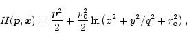
In this section we shall concentrate on some geometrical remarks concerning the
Hamiltonian corresponding to the logarithmic potential
Next we study the problem of representation of the phase space.
From (17) we note that for all
![]() ,
,
![]() defines a compact level of energy which can be seen as
defines a compact level of energy which can be seen as
![]() .
Indeed, for small
.
Indeed, for small ![]() one can keep the dominant terms
one can keep the dominant terms

Now let us pass to general values of ![]() .
Denote by
.
Denote by
![]() and define
and define
![]() which is analytic for any
which is analytic for any
![]() .
Then we introduce
.
Then we introduce

![\begin{figure}
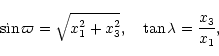
{$(x,p_x)\to (x_1,x_3)\to (\varpi,\lambda);\\ \, D\equiv\sin\varp...
...{H1686f9.ps}\par\includegraphics[angle=-90,width=7.3cm]{H1686f10.ps}\end{figure}](/articles/aas/full/2000/20/h1686/img238.gif) |
Figure 5:
Sketch of the transformation from the xpx to x1x3-plane
and to angles
|
A simple way to use these variables is as follows. All orbits intersect
transversally, for instance, y=0 except the x-axis periodic orbit which is
always contained on this plane and appears as the boundary of this surface of
section,
x12+x32=1 or
![]() - see Fig. 5.
One can identify the points in the boundary to a single point. Points
(x1,x3) such that
x12+x32<1, represent an open disc so that,
identifying the boundary to a single point, we obtain a 2D sphere
- see Fig. 5.
One can identify the points in the boundary to a single point. Points
(x1,x3) such that
x12+x32<1, represent an open disc so that,
identifying the boundary to a single point, we obtain a 2D sphere ![]() .
By
definition we send the origin
(x1,x3)=(0,0) to the south pole (SP) and the
boundary
x12+x32=1 to the north pole (NP). As it could be also used the
section x=0 and because in this case the boundary corresponds to the y-axis
periodic orbit,
x22+x42=1, we are interested in doing the mentioned
identification with suitable symmetry properties.
.
By
definition we send the origin
(x1,x3)=(0,0) to the south pole (SP) and the
boundary
x12+x32=1 to the north pole (NP). As it could be also used the
section x=0 and because in this case the boundary corresponds to the y-axis
periodic orbit,
x22+x42=1, we are interested in doing the mentioned
identification with suitable symmetry properties.
Given, for instance, x1 and x3 on the section through y=0, we define the
angles
![]() and
and
![]() as (see Fig. 5)
as (see Fig. 5)
Hence the "natural'' space to represent the full dynamics is ![]() .
Periodic
orbits along the axes appear at the poles and the "pendulum-like oscillations''
for loops fit on this sphere. One can also understand this representation by
looking back to Fig. 1 or Fig. 4. Points with
.
Periodic
orbits along the axes appear at the poles and the "pendulum-like oscillations''
for loops fit on this sphere. One can also understand this representation by
looking back to Fig. 1 or Fig. 4. Points with
![]() and
and ![]() are identified. In this way we obtain a cylinder. Then
points on the upper curve (1:1 direct periodic orbit) are identified to a single
point, as well as points on the lower curve (1:1 retrograde periodic orbit).
The cylinder becomes
are identified. In this way we obtain a cylinder. Then
points on the upper curve (1:1 direct periodic orbit) are identified to a single
point, as well as points on the lower curve (1:1 retrograde periodic orbit).
The cylinder becomes ![]() and then it is turned to have (0,0) and
and then it is turned to have (0,0) and
![]() at the SP and NP respectively. But note that in this case the
pendulum oscillations, as described in Sects. 2.1 and 2.2,
correspond to boxes.
at the SP and NP respectively. But note that in this case the
pendulum oscillations, as described in Sects. 2.1 and 2.2,
correspond to boxes.
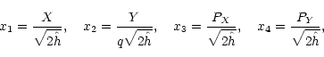
For completeness we list the transformation in case the
formulation (16) is desired. Let then, for instance, (x,px) be the values in
the y=0 surface of section with, say, py>0, unless we are at the boundary.
Compute first
![]() ,
PX=px/p0,
,
PX=px/p0,
![]() and then
and then
Figure 6 displays, for q=0.75,
![]() and h=-0.4059 (similar to
Fig. 1 (right) but for different variables) the cross section x=0.
The NP, that for this section corresponds to the unstable y-axis orbit,
is seen as an hyperbolic point inside a gross stochastic layer. The SP, that
corresponds to the x-axis orbit, also appears as an hyperbolic point, because
for this value of q the latter orbit is unstable. Note the 2-periodic
orbit
and h=-0.4059 (similar to
Fig. 1 (right) but for different variables) the cross section x=0.
The NP, that for this section corresponds to the unstable y-axis orbit,
is seen as an hyperbolic point inside a gross stochastic layer. The SP, that
corresponds to the x-axis orbit, also appears as an hyperbolic point, because
for this value of q the latter orbit is unstable. Note the 2-periodic
orbit![]() that bifurcates from the x-axis orbit that
gives rise to the banana orbits. The other elliptic points on the northern
hemisphere correspond to the 1:1 periodic orbit (direct and retrograde).
Therefore "pendulum-like'' oscillations correspond to loops while rotations to
boxes. In other words, for boxes,
that bifurcates from the x-axis orbit that
gives rise to the banana orbits. The other elliptic points on the northern
hemisphere correspond to the 1:1 periodic orbit (direct and retrograde).
Therefore "pendulum-like'' oscillations correspond to loops while rotations to
boxes. In other words, for boxes, ![]() ranges from 0 to
ranges from 0 to ![]() while for
loops,
while for
loops, ![]() is confined to some subinterval of
is confined to some subinterval of ![]() .
For a better
visualization, orbits in the "hidden'' part of the sphere (SP and almost all the
southern hemisphere) were drawn with much less points.
.
For a better
visualization, orbits in the "hidden'' part of the sphere (SP and almost all the
southern hemisphere) were drawn with much less points.
![\begin{figure}
\par\includegraphics[width=58mm,clip]{figure6.ps}\end{figure}](/articles/aas/full/2000/20/h1686/img255.gif) |
Figure 6:
Surface of section x=0 on the sphere
|
Copyright The European Southern Observatory (ESO)