4 Polarimetric sensitivity and noise estimations

Several tests have been performed to assess the noise in the data. We have measured three different types of noise. None of them includes systematic errors. We anticipate that with an improved setup those errors will disappear, or at least will be greatly diminished in the future. They have been discussed in previous sections: differences in the equivalent widths for each path, etc. The noise discussed here is that which remains if those systematic errors were not present.

4.1 Photon noise

We have measured the photon noise per pixel using the continuum region around the Fe I line at 5576 Å (data obtained on August 23rd, see Table 1). One hundred images of the disk centre for the Stokes V parameter were obtained at around 7:50 UT. The best way to measure photon noise is to compare two images identical except for the noise. As an approximation to this ideal we compared each image with the next one. But solar surface details were visible in the images, therefore we created two mean images by adding the odd and even numbered images respectively. The final images are free from solar features and comparison is done between the nearest images possible. A mean profile of the selected continuum region was taken for each mean image by adding the profiles along the slit. At this point, each one of the mean profiles contains $I + \delta _i$ (i=1,2): a common signal Iand an added noise $\delta _i$ . The ratio of the two profiles gave us (neglecting second order terms):

$\begin{displaymath}\frac{I + \delta _1}{ I + \delta _2}= 1 - \frac{\delta _2 - \delta _1} {I}.\end{displaymath}$

The mean value of this ratio is therefore 1 if the noise is well distributed around zero. The standard deviation of the ratio corrected for the number of images and the number of profiles along the slit (used to generate the mean profile) gives the noise per pixel. The resulting measured value is $\sigma = 2.4~10^{-3}$ . This value is consistent with a constant of 250 e^-/ADU (Analog--Digital Unit), as defined by the CCD's chipset constructor.

4.2 Polarimetric noise in the continuum

Next, we searched for the error in the continuum region in the reduced images of Stokes I, Q, U and V. The same 100 images of the disk center at 5576 Å were used for this purpose, but after reducing them as explained in previous sections and obtaining the Stokes parameters by simple addition and substraction. Each set of profiles from the four resulting images for the Stokes parameters was interpreted as a sole statistical variable. No consideration was made about how they had been obtained. The continuum in Q, U, V should show a null signal plus an error. In practice we observed a mean signal of 2 10^-4indicating a problem with the normalization of the continuum signal from the two paths. The standard deviation of each one of the images in the selected region of the continuum is shown in Fig. 6.

$\begin{figure} \psfig{file=fig6.ps,width=\hsize}\hfill \end{figure}$

Figure 6: Standard deviations measured in the continuum around the Fe I line at 5576 Å in the Stokes signals from a series of images of the disk center. The 3% of Stokes I is due to residual solar surface granulation (the telescope was randomly displaced during the exposures). The values in the other Stokes parameters are an indication of the photon noise and the errors accumulated in the data reduction process

In Stokes I the obtained value of around 3% is due to residual solar granulation(the telescope was randomly displaced during the exposures). Excepting this, the other 3 Stokes parameters show a common standard deviation for the whole series of images of approximately 3 10^-3 of the intensity of the continuum. This noise is slightly higher than the measured photon noise. For an exposure time of 300 ms, this number gives the polarimetric sensitivity of the instrument at the moment of the observations (August 1998).

4.3 Polarimetric noise in the lines

The previous measurement was done in the continuum in the disk center and near a line not sensitive to the magnetic field. We also wanted to obtain a value for the noise in a magnetically sensitive line in the presence of field. We used the PCA techniques for this purpose (Rees et al. 1999) and applied them to the series of 74 images taken on August 22nd for the spectral domain around the 6301 Å Fe I line. Some 14000 profiles for each one of the Stokes parameters were extracted from this series and used to create a database, from which PCA procedures derived 4 sets of eigenprofiles, one for each Stokes parameter. We also obtained the singular values associated with each one of the eigenprofiles. These singular values are an indication of the quantity of information contained in the respective eigenprofiles. For instance, Fig. 7 shows the ten first singular values obtained for Stokes Q. The entire set of eigenvalues represents the total information contained in the whole set of Q profiles extracted from the referred data. In the figure, the eigenvalues have been normalized to the sum of all the singular values, and its interpretation is very easy. For example the first eigenprofile contains on average 60% of the information present in each profile of the set taken into consideration. In fact it can be shown that this first eigenprofile is the mean profile of the set. The second eigenprofile will account for 17%, the third for 7% and so on. In total, 97% of the information contained in any particular profile can be reproduced by an adequate combination of the 10 first eigenprofiles.

$\begin{figure} \psfig{file=fig7.ps,width=\hsize}\hfill \end{figure}$

Figure 7: The ten first singular values of the set of Stokes Q profiles for the spectral region around 6301 Å from the observations of August 22nd. They have been normalized to the sum of the whole set of eigenvalues. As explained in the text, the value represents the amount of information contained on the respective eigenprofile. The continuous line is for clarity purposes only

The form of the curve in Fig. 7 gives us also an indication of what kind of information each eigenprofile is taking into account. PCA does not make the difference between signal and noise, but it concentrates the organized patterns in the data in a few singular values: the bigger ones. To reproduce the non-organized part of the data (i.e. noise and singular physical configurations) PCA require a lot of eigenprofiles. The respective singular values (the ones with higher indices) will therefore have similar values, indicating similar amounts of information. The curve with the singular values becomes flattened when the respective eigenprofiles are reproducing noise and not signal. In that sense PCA behaves similarly to a Fourier transform, where the noise is concentrated into the high frequencies, but it is much more efficient in distinguishing it. A more detailed account of the properties of this mathematical technique can be found in the book Numerical Recipes (Press et al. 1988), or in the papers by Hansen (1992), Hansen et al. (1992) and Hansen & Prost O'Leary (1993). For an application of this technique to solar and stellar spectral profiles, see Rees et al. (1999).

Back to our noise measurements, ten eigenprofiles are more than enough to reproduce the signal in the data discarding noise. However, to test the noise, we have reconstructed every profile present in the referred set with a combination of up to 25 eigenprofiles, and calculated what was the residual left. The results are presented in Figs. 8 and 9.

$\begin{figure} \psfig{file=fig8.ps,width=\hsize}\hfill \end{figure}$

Figure 8: Standard deviation (in % of the continuum signal) of the differences between the whole set of observed profiles and its reconstruction using a variable number of eigenprofiles. The continuous line is for clarity purposes only. The curves flatten from the moment they are reproducing noise. No more than 10 eigenprofiles suffice to take into consideration most of the information contained in the profiles

$\begin{figure} \psfig{file=fig9.ps,width=\hsize}\hfill \end{figure}$

Figure 9: Means (in % of the continuum signal) of the differences between the whole set of observed profiles and its reconstruction using a variable number of eigenprofiles. The continuous line is for clarity purposes only. The means go to zero when the residuals are just white noise. Once more (see previous figure) we see that at most 10 eigenprofiles are necessary to reproduce the information contained in the whole set of profiles

$\begin{figure} { \psfig{file=fig10.ps,width=3.5cm} } \end{figure}$

Figure 10: Image of the continuum for NOAA-8307 on August 22th (see the text). The image is $125\times 243$ pixels, each one spanning 0.4 $^{\prime \prime }$

Once more we see in these figures that the first eigenprofile suffices to reproduce each one of the observed profiles within 1 to 3% of the signal of the continuum. This is however not enough and between 5 and 10 eigenprofiles must be used to flatten the four standard deviation curves and drive the mean error to 0 (indicating a well centered noise). The error committed in the reconstruction without noise is of 4 10^-3 approximately, except for Stokes I which is kept at levels of 8 10^-3 for such a small number of eigenprofiles. These two numbers give the polarimetric noise level in the lines in the presence of signal.

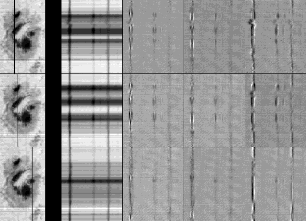
$\begin{figure} {\hspace{6cm} \psfig{file=fig11.ps,width=18cm} } \end{figure}$

Figure 11: The continuum image at left indicates the slit position for which the four Stokes parameters are shown (I,Q,U and V from left to right) for the spectral region around 6301 Å

$\begin{figure} {\hbox{\psfig{file=fig12.ps,width=15cm} }} \end{figure}$

Figure 12: The same as Fig. 11 except for the spectral region around 6149 Å

The profiles considered in the series of data include all the polarization signals of the observed spot for two magnetic-sensitive lines and two telluric lines. The obtained noise values are slightly higher (except for intensity for which it is clearly bigger) than those measured in the continuum. This is not surprising, as there is less signal in the lines than in the continuum, and furthermore, the data comes from a scan over a sunspot (while the continuum measurements were done for data taken on the disk center and in the quiet sun) so the photon noise is also higher. Hence the obtained result is consistent with the previous measurements.

**Table 3:** Noise in data
Photon Noise	2.4 10^-3
Polarimetric sensitivity in the continuum	3 10^-3
Polarimetric sensitivity in the lines	3-4 10^-3

4.4 Summary

The three noise measurements, which we have summarized in Table 3, are consitent with each other, and we can conclude that the photon noise level was under 3 10^-3 and that a polarimetric sensitivity of 3 to 4 10^-3 of the intensity of the continuum was available at the moment of these observations. It is very important to note that these measurements do not take into account systematic errors.

Among these systematic errors we indicate the following:

The observed difference between the equivalent widths for the two paths, probably due to the presence of polarized scattered light in the spectrograph;
The errors in the correction of the spatial and temporal gains per pixel;
The errors in the correction of the geometry between the two cameras;
And the errors in the polarization analyser, which will induce crosstalk among the Stokes parameters.

The first one is the most conspicuous in the reduced data and must be the object of a thorough test for subsequent observations. The last one is undoubtedly present, but the actual data does not allow a calibration nor even an estimation of this effect. Without such a calibration the expected residual instrumental polarization due to stresses in the entrance window may not be removed.

$\begin{figure} \par\psfig{file=fig13.ps,width=\hsize}\hfill \end{figure}$

Figure 13: The 4 Stokes parameters for a point of the first slit image in Fig. 11 at the spectral region around 6301 Å. Note the small inversion in the V profile center, probably due to anomalous dispersion. Note also the asymmetries in the Stokes profiles; they should be compared with those in the profiles of the same slit position shown in Fig. 14

$\begin{figure} \psfig{file=fig14.ps,width=\hsize}\hfill \end{figure}$

Figure 14: Asymetries in the profiles are evident at this point of the slit extracted from the first image in Fig. 12 in the spectral region around 6149 Å. To be compared with the ones found in Figs. 13 and 15

$\begin{figure}\psfig{file=fig15.ps,width=\hsize}\hfill \end{figure}$

Figure 15: Another set of Stokes profiles for the spectral region near 6149 Å extracted from the same slit as previous figure. Note the inverted asymetries relative to that previous figure

Up: First results from THEMIS mode