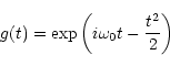
The Morlet wavelet gives the smallest time-bandwidth product [Lagoutte et al.1992].
![]() is a phase constant (in the present study
is a phase constant (in the present study
![]() = 5). For large
= 5). For large
![]() the frequency
resolution improves, though at the expense of decreased time resolution.
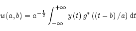
The dilation parameter may be considered as equivalent to the frequency of
the analyzed signal, while the translation parameter corresponds to the time
elapsed along the analyzed sample.
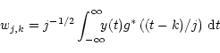
In practice, for analyzing a discrete-time signal y(ti)
we sample the continuous wavelet transform on a grid in the
time-scale plane (b,a) by choosing a=j and b=k where
j and k are integers. That is we compute wavelet coefficients
the frequency
resolution improves, though at the expense of decreased time resolution.
The dilation parameter may be considered as equivalent to the frequency of
the analyzed signal, while the translation parameter corresponds to the time
elapsed along the analyzed sample.
In practice, for analyzing a discrete-time signal y(ti)
we sample the continuous wavelet transform on a grid in the
time-scale plane (b,a) by choosing a=j and b=k where
j and k are integers. That is we compute wavelet coefficients
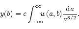
Since the wavelet transform is an over-complete representation of the original signal (a one-dimensional signal is transformed to the two-dimensional plane) there are many possibilities for reconstructing the signal. One way is to use a discrete version of Morlet's formula
 |
(6) |
Note that the original signal's low-pass (DC) component is lost in the transform.
In the present study dilation number 1 corresponds to the highest frequency (a half of sampling rate). The highest dilation number corresponds to the lowest observable frequency.
Copyright The European Southern Observatory (ESO)
![\begin{displaymath}G(\omega) = \sqrt{2\pi} \exp\left[-\frac{\left(\omega - \omega_{\mathrm{0}}\right)^2}{2}\right]\cdot
\end{displaymath}](/articles/aas/full/1999/19/h1509/img16.gif)