 |
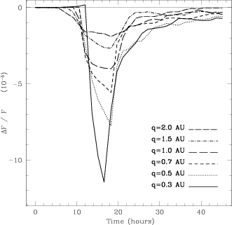
Figure 3: Same as Fig. 2. Here all the parameters are the same except that the star is always taken to be a G type star and the periastron distance is allowed to vary form 0.3 AU to 2.0 AU. Of course, the amplitude of the variation significantly increases when the periastron decreases |
The parameter space is a 6-dimensional space (size distribution, stellar
type, P0, q, ![]() ,
b). For each parameter
the range of value has been sampled at several positions. The number
of positions for each parameter is (3, 5, 5, 6, 15, 6). In fact, comets
at 2 AU from a K type star or farther than 0.7 AU from a M type star
are beyond the water ices sublimation limit and should not evaporate.
The models with
,
b). For each parameter
the range of value has been sampled at several positions. The number
of positions for each parameter is (3, 5, 5, 6, 15, 6). In fact, comets
at 2 AU from a K type star or farther than 0.7 AU from a M type star
are beyond the water ices sublimation limit and should not evaporate.
The models with
![]() have not been calculated
for A stars because of computer-time limitation.
Finally, we obtain 33480 different models for the M, K G, F, and A stars
(
have not been calculated
for A stars because of computer-time limitation.
Finally, we obtain 33480 different models for the M, K G, F, and A stars
(
![]() ).
).
Each resulting model is given a name composed by the names of the parameters
and underscores. For example, with the dust size distribution so-called
"50'', a comet orbiting a G type star with a production rate of
105 kg s-1 and a periastron at 1 AU located on the line of sight
(![]() ,
b=0), the model-name is "50_G_50_10_00_00''.
The name-substrings corresponding to parameters values are given in
Table 2.
,
b=0), the model-name is "50_G_50_10_00_00''.
The name-substrings corresponding to parameters values are given in
Table 2.
Each file has an header giving the value of the parameters used in the simulation and an 8-columns table. This table gives the light variation as a function of the time during 45 hours with a time-step of 1.5 hours. The first column gives the time in days relative to the periastron passage. The second column gives the maximal fraction of the stellar light extinct by the comet dust cloud. This maximal extinction is obtained by considering a wavelength of observation shorter than the size of any dust particle. The Cols. 3 to 5 give the fraction of the stellar light extinct by the comet at wavelengths 400, 800 and 2200 nm, roughly corresponding to observations in the B, R and K bands. The Cols. 6 to 8 give the fraction of the stellar light scattered by the dust at the same wavelengths. An example of such a table is given in Table 3. A resulting light curve is simply obtained by the addition of the extinction to the scattering at the corresponding wavelength.
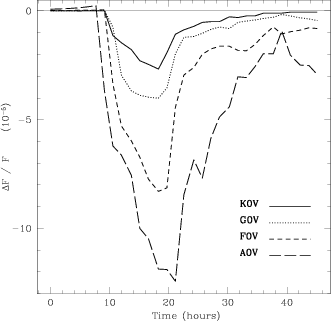
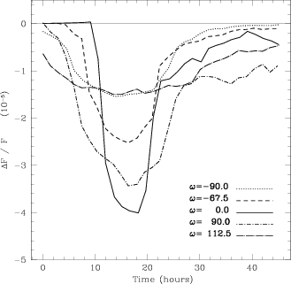
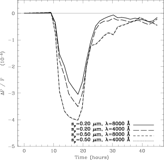
To illustrate the effect of the parameters, we take as an example the light curve corresponding to the model "50_G_50_10_00_00'' and we vary one of the parameters. The resulting light curves are plotted in Figs. 2 to 6. We see that, at a first order, the amplitude of the variation is proportional to the dust production rate and inversely proportional to luminosity/mass ratio.
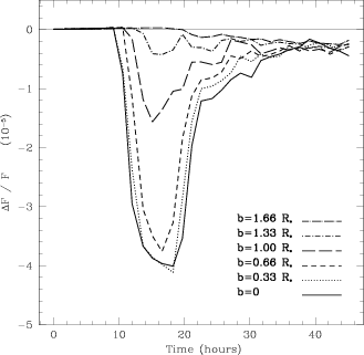 |
Figure 5: Same as previous figures. Here the impact parameter varies up to 1.66 times the stellar radius |
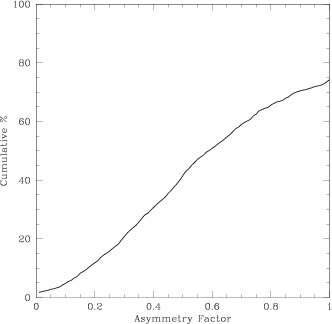 |
Figure 7: Plot of the weighted cumulative percentage of light curves with an asymmetry factor smaller than a given value. The asymmetry factor is defined in Sect. 4. Each light curve is given a weight as a function of the periastron q, the production rate P0 and the type of the central star. We use d n(q)=q0.3dq and d n(P0)=P0-2.25dP0 (LVF 99). We consider the proportion of each type of star for a magnitude limited sample of single main sequence stars: K 2%, G 10%, F 31%, A 57%. The maximum percentage does not go up to 100% because the asymmetry factor can be larger than 1. This happens when the scattering dominates the extinction and consequently the star brightness increases, then some points of the photometric variation are significantly positive. We see that the asymmetry factor is smaller than 0.1 for 5% of the light curves, it is smaller than 0.15 in 8% of the cases and smaller than 0.2 in 12% of the cases |
Copyright The European Southern Observatory (ESO)