3 Observations and data reduction

In order to investigate the low frequency part of the spectra of Subsample Two sources we set up a programme of flux density measurements at low frequency with a high resolution facility. We used MERLIN at 408 MHz because of its superior resolving capability -- $1\hbox{$^{\prime\prime}$}$. The observations were carried out in the period from November 1994 until January 1995 and each source was typically observed twice (with different hour angles) for about 15 minutes per scan.

Such short snapshots cannot be used to produce reliable maps with MERLIN, since the aperture coverage is too sparse. Confusion is a significant effect at this low frequency and therefore fringe-frequency vs. delay (FFD) plots were used to separate confusing sources from the central target source (see e.g. Walker 1981). Since the data were not phase-calibrated the coherence time is limited to a few minutes. By taking $128\times 4$ second sub-samples of the data and Fourier transforming them in both time and frequency, a "map'' of the field surrounding the source can be produced whose axes are fringe-frequency and delay. The target source will have close to zero fringe-frequency and delay, since its position is well known from the JVAS survey, and appear at the centre of the "map'', while confusing sources will be offset from the centre. The flux density of the target source was determined from the central peak in the FFD map. The FFD plots were inspected visually; the detection threshold in a single plot was set at $3\sigma$ and flux density values were only listed if the target was detected in two or more plots. In all cases, the values determined from the FFD plots were consistent with simple averages of phase-calibrated data on individual baselines calculated using the Astronomical Image Processing System (AIPS). The flux density scale was determined using observations of 3C 286, for which the Baars et al. (1977) value was used.

 

Table 2: Subsample Two -- flux densities of sources at 408 MHz

 

Table 2: continued

Explanation of ID field is given in Table 1.

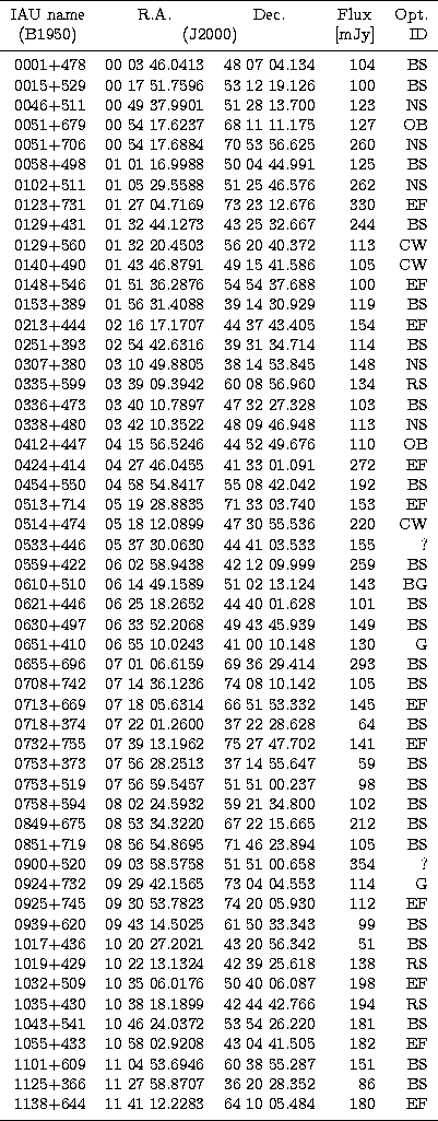
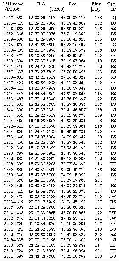
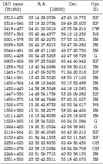
In Table 2 we report the results of successful measurements of 408 MHz fluxes for 98 sources from Subsample Two along with their JVAS positions rounded to 1 milliarcsecond and our identifications made using POSS. Interference and other problems at other sites resulted in the loss of data for the remaining 27 sources. They are listed in Table 3. The flux density values given in Table 2 resulted from averaging the measurements over all baselines involving the Defford or Knockin telescopes (6 or 8 baselines, depending on whether the Lovell telescope was used or not) and in both LL and RR polarisations. Shorter baselines were not used because they provide insufficient resolution in delay or fringe-frequency to separate the confusing sources; additionally the use of longer baselines reduces any contribution from large-scale halos seen around some GPS sources. The longest baselines involving the Cambridge telescope were not used because interference limited the useful bandwidth to 1.5 MHz, rather than the 4 MHz used elsewhere. Because baseline combinations and the volume of data per source varied form source to source the errors range form 10 to 30 mJy.

 

Table 3: Subsample Two -- sources not measured at 408 MHz

Explanation of ID field is given in Table 1.