2 Analysis of the data

When a galaxy is observed with low spatial resolution relative to the gas extension, the HI maps show a roughly gaussian distribution. When the spatial resolution grows, some structures appear, such as inner and external rings, several concentrations, etc. For high resolution observations, fine structures such as spiral arms, gas shells, "holes" in the HI distribution, etc., start to be resolved. In all cases, the observed distribution of the gas is the convolution of the real one with the antenna response.

We have collected the maps of the integral HI density distribution in the catalogue of Paper I. As the main parameter of the sample we are dealing with is the real extension of the gas, we ought to make the deconvolution. Then, among these maps, we kept those whose contour lines show no detailed structures which would complicate a further analysis. In this way, we can apply a simplified gaussian model for the gas distribution that masks particular details, asymmetries and some large-scale features that are common in most galaxies.

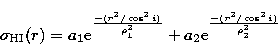
It is known that the real HI distribution often shows a central depression, especially in early spiral galaxies (Roberts 1975; Sersic 1980). It is convenient that the model representative of the gas distribution takes this fact into account. A frequently-used symmetrical model which gives a useful rough representation for most spiral galaxies is the sum of two gaussians (Shostak 1978; Hewitt et al. 1983). One gaussian distribution of HI gas may work for irregular galaxies, because of their flat gaseous disk distribution. Thus, we have adopted one and two gaussian models of the HI distribution for irregular and spiral galaxies, respectively, which are represented by the following expression:

$$\sigma_{\rm HI} (r) = a_{1} {\rm e}^{ \frac{-(r^{2}/\cos^{2}... ...} + a_{2} {\rm e}^{ \frac{-(r^{2}/\cos^{2} i)}{\rho_{2}^{2}}}$$ (1)

where r is the radial distance, i is the inclination of the galaxy and a₁, a₂, $\rho_{1}$ and $\rho_{2}$ are model parameters, with a₂ = C₁ a₁ ; $\rho_{2} = C_{2} \rho_{1}$.
For a one-gaussian model, a₂ = 0 (C₁= 0). For a two-gaussian model, Hewitt et al. (1983) adopt C₁= -0.6 for the relative strength of the gaussians, which produces a deeper central depression than the Shostak model (1978) with C₁= -0.3. We use C₂= 0.5 for the relative width of the gaussians. The model parameter a₁ is concerned with the strength of the emission. We have normalised the intensity of emission to the central values on the maps. The $\rho_{1}$ parameter is the factor that radially compresses or expands the HI distribution, and is basically the parameter on which the fit depends.

In order to make the fit, we first determined the major axis of the gas distribution from the map. On this major axis, we obtained the radial distances (r) and the observed HI surface density at these distances. It is worth to noting that the HI major axis may not be coincident with the optical axis. In fact, this issue lead us to consider only the papers with maps of the total distribution of the gas emission, and reject those papers with observations along only one axis of the galaxy.

The expression (1) was convolved with the beam width of the telescope used in the observation, which was supposed gaussian as well. This convolution must reproduce the distribution of the HI surface density observed in the map. Then, we iteratively vary $\rho_{1}$ in expression (1) until the best mean least square fit between the calculated and observed values is achieved. With respect to the relative strength of the gaussians, represented by the C₁ parameter, we took its values at -0.6 or -0.3, depending on which gave the best fit to the observations. The result was that for galaxies with morphological type earlier than 4, the number of objects that best fit with C₁ = -0.3 is approximately the same as the one with C₁ = -0.6. However, for later-type galaxies, the number of best fits with C₁ = -0.3 is remarkably large. This result may be in agreement with the fact that the central depression in the HI distribution seems to be less pronounced in late-type systems, which possess small bulges.

For comparison with optical isophotal diameters, the best-fit model is used to compute the HI isophotal diameter, then corrected by beam and inclination effects. The isophotal diameters are defined according to a particular isophote. By inspection of the data, we find that the best sensitivity reached in the observations is, in most cases, 2.5 10¹⁹ at cm^-2, and we have adopted this value for estimating the HI isophotal diameter ($D_{\rm HI}$). We only kept those galaxies measured until a surface density less or equal to 15 10¹⁹ at cm^-2, because we have found that the extrapolation is not valid for larger values.

In Table 1, we have listed the galaxies that make up the sample that we use for the subsequent analysis. The optical parameters are extracted from the LEDA catalogue (Lyon-Meudon Extragalactic Database, first and second edition). First entries to the table are:
Column 1: Galaxy name.
Column 2: Alternative name of the galaxy.
Column 3: Optical isophotal diameter measured to the surface brightness level of 25 mg/[]'' corrected for galactic and internal absorption (D₀), in arc minutes.
Column 4: Morphological type.
Column 5: Inclination, in degrees.
Column 6: Distance, in Mpc. When the distance is uncertain, the extreme assumed values are quoted. See following discussion.
Column 7: The linear diameter A(0) in kpc, from Cols. 3 and 6.
Column 8: HI mass, $M_{\rm HI}$, in 10⁹ M₀. The adopted values of $M_{\rm HI}$ are discussed in Sect. 4.
Column 9: Mean apparent surface density of HI, $\rho_{\rm HI}$, in 10²¹ at cm^-2, from Cols. 7 and 8.
Column 10: Mean real surface density, $\Sigma_{\rm HI}$, in 10²⁰ at cm^-2, from Col. 8 and the HI isophotal diameter, $D_{\rm HI}$ (see Col. 3 of second entry).
Second entries to the Table are:
Column 1: Telescope used in the observation. (see Paper I for the abbreviations).
Column 2: Beam width of the telescope, in arc minutes.
Column 3: Ratio between the HI and optical isophotal diameters, $D_{\rm HI}/D_{0}$.
Column 4: References. The reference numbers are the same as those of the catalogue of Paper I.