Appendix

The derivation of estimates for the uncertainties in flux S, position $\eta$, and width $\theta$ of a one-dimensional gaussian brightness distribution centered at $\eta = 0$ and sampled at locations $\eta_j = \pm j\cdot \theta_B/2$ ($j=0\ldots N$,$\;\theta_B$ is the beamwidth) with additive noise $\epsilon$ of zero mean and variance $\sigma^2_N$

$$B_j(S,\theta) = S \exp\,(-((\eta_j-\eta)^2/2\theta^2))_{\vert _{\eta=0}}+ \epsilon\,(\eta_j,0,\sigma^2_N)$$ (8)

requires the use of non-linear regression. A Gaussian profile is indeed non-linear in $\eta$ and $\theta$ according to

$$\delta B/\delta \eta \sim \eta \,B\,\theta^{-2} \mbox{\hskip... ...hskip 3mm} \delta B/\delta \theta \sim \eta^2 \,B\,\theta^{-3}.$$ (9)

Though non-linear regression is required to derive estimates of the uncertainties in S, $\eta$ and $\theta$, we used an approach suggested by the iterative Gauss-Newton method (Bates & Watts 1988) to derive a linear approximation to these estimates in the limit of high signal-to-noise ($=S/\sigma_N$). In this case the one sigma confidence limit for the position $\eta$ in the limit of high N can be written to

$$\sigma^{-2}_\eta \cong \sigma^{-2}_N \cdot \lim_{N \rightarrow \infty} \sum_{j=0}^N (\delta B_j/\delta \eta_j)^2$$ (10)

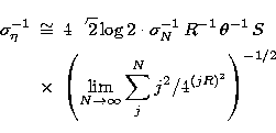
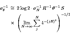
with similar expressions for $\sigma^{-2}_S$ and $\sigma^{-2}_\theta$.According to equation (10) the uncertainties in S, $\eta$ and $\theta$ for the gaussian brightness distribution B are given by

$$\sigma_S^{-1} \cong \sigma^{-1}_N \cdot \left(\lim_{N \rightarrow \infty} \sum_j^N j^4/4^{(jR)^2}\right)^{-1/2}$$ (11)

$$\begin{eqnarray} \sigma_\eta^{-1} &\cong & 4\sqrt{2}\log 2 \cdot \sigma^{-1}_N\,... ...im_{N \rightarrow \infty} \sum_j^N j^2/ 4^{(jR)^2}\right)^{-1/2} \end{eqnarray}$$ (12)

$$\begin{eqnarray} \sigma_{\theta}^{-1} &\cong & 2\log2 \cdot \sigma^{-1}_N\, R^{... ...eft(\lim_{N \rightarrow \infty}\sum_j^N 4^{-(jR)^2}\right)^{-1/2} \end{eqnarray}$$ (13)

where $R = \theta_B/\theta$. Note that in the R=1 limit (i.e. an unresolved object) the uncertainties can roughly be estimated to $\sigma_S \cong \sigma_N$, $\;\sigma_\eta \cong (\theta_B/2)(\sigma_N/S)$ and $\sigma_\theta \cong \theta_B (\sigma_N/S)$. The errors in the estimates are reasonably small for samples with snr $\ge 10$. In analogy, statistical estimates for S, $\eta$ and $\theta$ according to the two-dimensional case were approximated to $\sigma_S \cong 0.7 \sigma_N$, $\;\sigma_\eta \cong (\theta_B/2)(\sigma_N/S)$ and $\sigma_\theta \cong \theta_B \sigma_N/S$ and found to be better than 20% for data with snr $\ge 10$.