2. The model

Fulle et al. (1995) have developed a probabilistic model able to estimate the dust flux on a probe, in a fly-by configuration (Fulle et al. 1995). To adapt the model to a rendez--vous scenario, the first relevant element to be considered is the similarity, in this case, of the probe and comet heliocentric velocities. The fly-by time scale is so short that changes occurring in the coma are negligible. On the contrary, the probe orbital period around the nucleus is generally so long that changes occurring in the coma, due to the variations of the sun comet distance, have to be accounted for. The main quantity measured by a dust collecting experiment is the dust fluence, i.e. the integral of the dust space density along the probe path. This is parametrized by the time, t, spent by the probe around the nucleus. Moreover, the dust space density in every point of the coma at a given time t depends on the time integral of the dust ejection from the nucleus occurred in the past: this past history is parametrized by the time , elapsed from dust ejection from the nucleus. It follows that the fluence comes from a double time integration. Thus, the time interval between ejection and impact on the probe is . If we are interested in the dust fluence collected by the probe during one orbit, the time t ranges between the starting time and , where P is the probe orbital period, while ranges from , corresponding to the comet aphelion (when the comet is assumed to be inactive) to the impact time t.

  
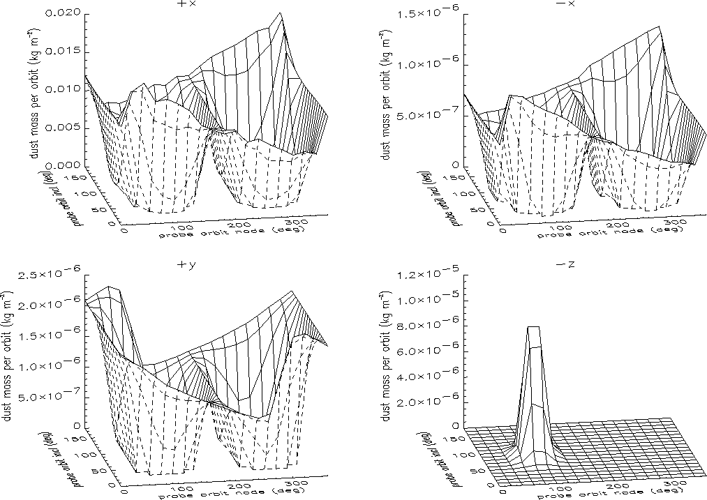
Figure 6: Dust mass per unit surface collected during a probe orbit for R = 50 km, starting sun-comet distance r = 1.762 AU, . Pointing directions: +x, -x, +y and -z

A fundamental quantity is the velocity vector of dust ejected from the inner coma that is required to impact the probe, . It depends on the dust ejection time, , the grain diameter, s, and the probe position along its orbit, which is determined by t and by the probe orbit geometry. Details for the computation of this vector were described by Fulle et al. (1995). By means of keplerian mechanics, from it is possible to compute the impact velocity vector projected in a probe reference frame, . Dealing with we face a second relevant difference with respect to a fly-by scenario. In this case, results always opposite to the probe motion and its absolute value is equal to the probe velocity, which is much higher then the dust velocity. In the case of an orbiting probe, such a trivial case never occurs and can be computed from the vectorial sum of the negative probe orbital velocity and the dust impact velocity. Among the grains impacting the probe, only those having a vector entering the acceptance angle of the dust collecting experiment contribute to the measured dust fluence.

The aim of our dust flux model is to compute the differential fluence, f(s), the cumulative fluence, h(m), the total mass collected per unit surface, , and the mass flux, . Thus, we have to consider , i.e. the number of particles inside the coma volume . Here, is the grain number loss rate of the comet, g(s) is the differential dust size distribution at the ejection and represents the ejection velocity vector distribution (which describes both the velocity absolute values distribution and the ejection anisotropies) of grains ejected inside the solid angle . The length is the radius of the dust shell ejected with velocity , for time intervals - between ejection () and impact (t) times - corresponding to anomalies smaller than (Finson & Probstein approximation, 1968). The differential fluence, f(s), is given by:

Here, the integration variable is replaced by and is the absolute value of the vector , if this vector enters the acceptance angle of the experiment, otherwise . From the differential fluence, we obtain:

   

r (AU) R (km) P (d) Fig. No

1.762 100 91 40 - - 2

1.762 100 91 40 120 10 3

1.762 100 91 40 100 90 4

1.762 100 91 40 120 60 5

1.762 50 32 40 - - 6

1.762 50 32 40 120 10 7

2.624 100 91 40 - - 8

2.624 100 91 40 120 10 9

1.762 100 91 80 - - 10

1.762 100 91 80 120 10 11

1.762 100 91 80 120 60 12

1.762 100 91 180 - - 13

1.762 100 91 180 120 10 14

1.762 100 91 180 100 90 15

1.762 100 91 180 120 60 16

1.762 50 32 180 - - 17

1.762 50 32 180 120 10 18

2.624 100 91 180 - - 19

2.624 100 91 180 120 10 20

  
Figure 7: Dust mass flux (left panel) and cumulated fluence (right panel) for R = 50 km, starting sun-comet distance r = 1.762 AU, , and . Pointing directions: +x (continuous line), -x (dot dashed line), +y (short dashed line), -y (long dashed line), and -z (three dot dashed line)

  
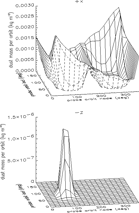
Figure 8: Dust mass per unit surface collected during a probe orbit for R = 100 km, starting sun-comet distance r = 2.624 AU, . Pointing directions: +x and -z

  
Figure 9: Dust mass flux (left panel) and cumulated fluence (right panel) for R = 100 km, starting sun-comet distance r = 2.624 AU, , and . Pointing directions: +x (continuous line), -x (dot dashed line), +y (short dashed line), -y (long dashed line), and -z (three dot dashed line)

(i) the dust mass per unit surface collected in a probe orbit

(ii) the cumulated fluence per unit surface, collected in a probe orbit

(iii) the dust mass flux per unit time and surface, collected in a probe orbit

where m, m and 10³ kg . For , we assume the following gaussian distributions:



where erf is the error function, is the most probable velocity, v₀ is the velocity dispersion, is the solar zenithal angle and is the ejection dispersion. Finally, the gas loss rate and the dust to gas ratio allow us to compute the dust mass loss rate and, then, during the comet orbit by means of g(s).